STAC, COG and Zarr: how to search satellite imagery in the cloud without downloading terabytes

In my first projects with Sentinel-2, getting the images was a manual job. On the Copernicus portal (the Open Access Hub, back then), I picked scenes by their thumbnail and downloaded a .zip of almost a gigabyte per scene. Then I unzipped it, browsed the .SAFE folder down to GRANULE/.../IMG_DATA and grabbed the .jp2 files of the bands I needed, usually two or three out of a package with more than a dozen. Often, only at that point did I see that the area of interest was covered in clouds. Much of the time went into downloading and organizing files, and the disk held far more data than the analysis used.

A Sentinel-2 scene covers about 110 × 110 km, and I almost always need a crop of a few kilometers. In a time series, with dozens of dates and several bands, the downloaded volume grows to tens of gigabytes just to analyze one city.

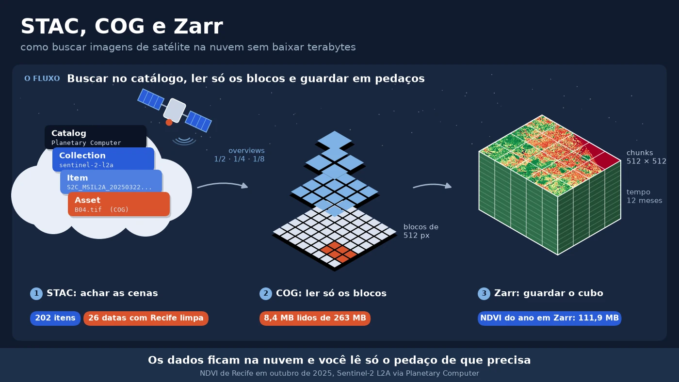
The data stays in the cloud and the code reads only the piece it needs. In this article, I show that path in practice, using Recife (a coastal city in northeastern Brazil) in 2025 as the example. We search for scenes in a STAC catalog, measure how many bytes actually leave a COG when we ask only for the city's area, build a monthly NDVI cube without downloading any full scene and store the result in Zarr and COG. The topic is one of the new chapters of the ebook 2.0. Here it gets real numbers.

It is worth stressing that we are not talking about Google Earth Engine here. It also processes in the cloud, but with its own catalog and API, and the code stays tied to the platform. The focus here is on open standards (STAC, COG and Zarr). The platforms we will use, Microsoft's Planetary Computer and Earth Search, which indexes the open data hosted on AWS, are company services, free to search and read, but they are not open. What is open is the Sentinel-2 data and the standard, and it is the standard that lets you switch providers, including to public catalogs such as ESA's Copernicus Data Space and INPE's Brazil Data Cube.

Three pieces that fit together

Before the code, it helps to separate the pieces, because each one solves a different problem.

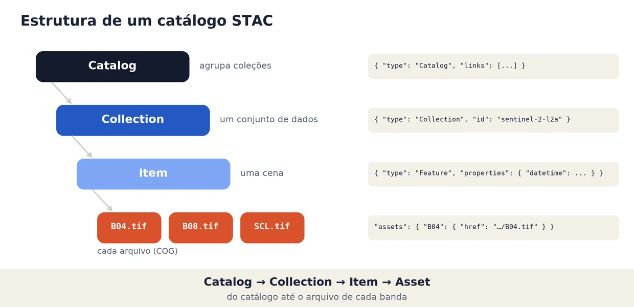
STAC (SpatioTemporal Asset Catalog) is the open specification that standardizes how to describe and search geospatial data in JSON. It has four levels. The Catalog is the entry point, the Collection groups a dataset (for example, all of Sentinel-2 level 2A), the Item describes a scene with geometry, date and properties, and the Assets are the item's files, one per band.

COG (Cloud Optimized GeoTIFF) is a regular GeoTIFF, organized in blocks (tiles) and with reduced versions of the image (overviews) embedded. Since the block index sits at the beginning of the file, a program can request over the internet only the bytes for the area and resolution it needs, using HTTP requests with a Range header. Any software that reads GeoTIFF also reads a COG.

Zarr stores multidimensional arrays (time × row × column, for example) in independent pieces, the chunks, each in a separate file or object. It is the natural format for data cubes and long series, where COG, designed for one 2D image per file, starts to get awkward.

In practice, STAC answers "where are the images I want", COG answers "how do I read only a piece of each image" and Zarr answers "how do I store the cube I built so I can read pieces of it later".

Searching for Recife's scenes in the catalog

We start with the STAC catalog of Microsoft Planetary Computer, which is free and requires no account to search. The search takes the collection, a rectangle in longitude and latitude (bounding box) and the period. Note that no pixel is downloaded here; only metadata comes back.

import pystac_client

BBOX = [-35.02, -8.15, -34.86, -7.95]  # Recife (lon/lat)

catalogo = pystac_client.Client.open("https://planetarycomputer.microsoft.com/api/stac/v1")

todas = catalogo.search(
    collections=["sentinel-2-l2a"],
    bbox=BBOX,
    datetime="2025-01-01/2025-12-31",
).item_collection()

limpas = catalogo.search(
    collections=["sentinel-2-l2a"],
    bbox=BBOX,
    datetime="2025-01-01/2025-12-31",
    query={"eo:cloud_cover": {"lt": 20}},
).item_collection()

print(len(todas), "cenas em 2025 sobre Recife")
print(len(limpas), "cenas com menos de 20% de nuvens")

item = limpas[0]
print("\nprimeiro item:", item.id)
print("nuvens (%):", item.properties["eo:cloud_cover"])
print("tile MGRS:", item.properties["s2:mgrs_tile"])
print("EPSG:", item.properties["proj:code"])
print("assets:", ", ".join(item.assets))
print("\nB04 ->", item.assets["B04"].media_type)

202 cenas em 2025 sobre Recife
7 cenas com menos de 20% de nuvens

primeiro item: S2C_MSIL2A_20250322T124311_R009_T25LBL_20250322T165113
nuvens (%): 6.142854
tile MGRS: 25LBL
EPSG: EPSG:32725
assets: AOT, B01, B02, B03, B04, B05, B06, B07, B08, B09, B11, B12, B8A, SCL, WVP, visual, safe-manifest, granule-metadata, inspire-metadata, product-metadata, datastrip-metadata, tilejson, rendered_preview

B04 -> image/tiff; application=geotiff; profile=cloud-optimized

The two searches took about seven seconds. The 202 scenes are 100 overpass dates, because Recife sits right on the border of two Sentinel-2 reference tiles (25LBL and 25MBM), and each overpass produces one item per tile. The type of the B04 asset already tells us the file is a COG (profile=cloud-optimized). And its address has the same folder structure I used to browse in the .zip (.SAFE/GRANULE/.../IMG_DATA/R10m/), except that it ends in .tif rather than .jp2. Planetary Computer converted the original JPEG 2000 bands to COG, and that conversion is what makes it possible to read only a piece of each one over the network.

With the classic filter of less than 20% cloud cover, 7 items on 5 dates remain. Recife's whole year fits into March, April and November.

eo:cloud_cover says nothing about your area

The eo:cloud_cover field is computed for the whole tile, about 12,000 km², much of it ocean in Recife's case. A scene can have 60% clouds overall and be clear exactly over the city, or the opposite.

To know what happens in the area that matters, we use the SCL layer (Scene Classification Layer), which ships with Sentinel-2 L2A and classifies each pixel as vegetation, soil, water, cloud, shadow and other classes. To keep the screening fast, we read the SCL at low resolution. At 200 m instead of the native 20 m, the reader uses the COGs' overviews and brings few bytes per scene.

import odc.stac
import planetary_computer

itens = [planetary_computer.sign(i) for i in todas]  # assina os links dos assets

scl = odc.stac.load(itens, bands=["SCL"], bbox=BBOX, resolution=200,
                    groupby="solar_day", chunks={}).SCL.compute()

com_dado = scl > 0                   # 0 = sem dado
limpo = scl.isin([4, 5, 6])          # vegetação, solo exposto, água
frac = limpo.sum(dim=["x", "y"]) / com_dado.sum(dim=["x", "y"])
print(f"SCL de {scl.sizes['time']} datas a 200 m ({scl.sizes['x']} x {scl.sizes['y']} px)")
print(f"datas com >= 50% de Recife limpa: {int((frac >= 0.5).sum())} de {frac.size}")

SCL de 100 datas a 200 m (90 x 112 px)
datas com >= 50% de Recife limpa: 26 de 100

Screening the 100 dates took 11 seconds. planetary_computer.sign appends a temporary access token to the links, required by Planetary Computer's storage. groupby="solar_day" merges the two tiles of the same overpass into a single date.

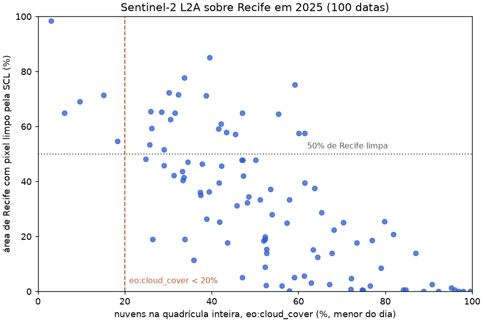
Each point is a date. The horizontal axis shows eo:cloud_cover (the lower of the day's two tiles) and the vertical axis, the fraction of Recife with clear pixels according to the SCL. The correlation exists (0.74), but the scatter is large. There are dates with 40% to 70% cloud over the scene that leave more than 60% of the city clear. With the criterion applied to Recife's area we keep 26 dates; with the scene filter, 5. That is 21 good dates the classic filter would throw away.

This does not make eo:cloud_cover useless. It is still good as a first cut, for example to discard scenes with more than 90% cloud before any reading. What does not work is using it as the final criterion for a small, cloudy area like the coast of northeastern Brazil. Since reading the SCL at 200 m costs seconds, it is worth screening on the area of interest whenever the series is short or the place is cloudy.

Reading only the bytes that matter from a COG

When we ask only for Recife's area, how much of the file actually crosses the network? To measure it, I opened the B04 band of the least cloudy scene of tile 25MBM, which covers almost the whole city, with a custom HTTP reader. GDAL, which sits behind rasterio, requests ranges of the file, and the reader makes one Range request for each range and adds up the bytes received.

class ArquivoHTTP(io.RawIOBase):
    """Arquivo remoto lido por requisições HTTP Range, com contador de bytes."""

    def read(self, n=-1):
        cab = {"Range": f"bytes={self.pos}-{self.pos + n - 1}"}
        dados = self.sessao.get(self.url, headers=cab).content
        self.pos += len(dados)
        self.bytes_lidos += len(dados)
        self.requisicoes += 1
        return dados
    # seek, tell e o HEAD inicial com o tamanho do arquivo estão no repositório


with rasterio.open("b04.tif", opener=opener) as src:   # opener devolve um ArquivoHTTP
    limites = transform_bounds("EPSG:4326", src.crs, *BBOX)
    janela = from_bounds(*limites, transform=src.transform)
    recife = src.read(1, window=janela)

The opener parameter of rasterio (from version 1.4 on) lets GDAL read through a Python object, which makes it possible to count the bytes. I did three reads, each opening the file from scratch.

arquivo B04: 262.9 MB, 10980 x 10980 px, uint16
blocos: [512, 512] | overviews: [2, 4, 8, 16] | compressão: deflate
só o cabeçalho: 5 KB em 112 requisições

janela de Recife: 1774 x 2221 px (3.3% da área da cena)
transferido: 8.4 MB (3.2% do arquivo) em 134 requisições

cena inteira em 1/16: 686 x 686 px
transferido: 0.8 MB (0.3% do arquivo) em 118 requisições

The file is 262.9 MB and is split into 484 blocks of 512 × 512 pixels, with four overview levels. Just to open it and learn the grid, GDAL read 5 KB. For Recife's window, which covers 3.3% of the scene's area, 8.4 MB were transferred, or 3.2% of the file. The cost of reading follows the requested area, not the file size. For an overview of the whole scene, at 1/16 of the resolution, 0.8 MB was enough, because the reader went straight to the overview instead of downsampling the 10980 × 10980 pixels.

The Python reader makes one request per range and is therefore slow (about 40 seconds for the window). It exists only to measure. Through GDAL's native HTTP reader, which merges neighboring ranges and keeps a cache, the same window arrived in 6.6 s and the reduced scene in 1.4 s, on my home connection.

Building the NDVI cube without downloading the scenes

With the 26 selected dates, we build the cube with odc-stac. It takes the STAC items, figures out the grid, reads only Recife's window from each COG and returns an xarray.Dataset with dimensions time, y and x. With chunks, reading becomes lazy. Nothing is read until .compute(), and dask processes block by block without needing the whole cube in memory.

cubo = odc.stac.load(
    itens_selecionados,                 # 54 itens das 26 datas
    bands=["B04", "B08", "SCL"],
    bbox=BBOX,
    resolution=10,
    groupby="solar_day",
    chunks={"x": 1024, "y": 1024},      # leitura preguiçosa com dask
)

# SCL: 4 vegetação, 5 solo exposto, 6 água (o resto é nuvem, sombra, sem dado etc.)
validos = cubo.SCL.isin([4, 5, 6]) & (cubo.B04 > 0)
# a partir da baseline 04.00 (jan/2022) o L2A soma 1000 aos números digitais
red = (cubo.B04.where(validos) - 1000) / 10000
nir = (cubo.B08.where(validos) - 1000) / 10000
soma = nir + red
ndvi = ((nir - red) / soma).where(soma > 0)    # água escura pode zerar o denominador

ndvi_mensal = ndvi.resample(time="1MS").median().compute()

The repository's cubo_ndvi.py also adds up the size of the full files and summarizes each month.

cubo em memória (se carregado inteiro): 1174 MB
arquivos completos de B04, B08 e SCL das 54 cenas: 27.11 GB

NDVI mensal calculado em 219 s
jan: 1 data(s),  50.8% da área com ao menos um pixel limpo, NDVI médio 0.311
fev: 0 data(s),   nan% da área com ao menos um pixel limpo, NDVI médio nan
mar: 2 data(s),  86.6% da área com ao menos um pixel limpo, NDVI médio 0.408
abr: 2 data(s),  99.4% da área com ao menos um pixel limpo, NDVI médio 0.454
mai: 1 data(s),  64.4% da área com ao menos um pixel limpo, NDVI médio 0.406
jun: 2 data(s),  76.5% da área com ao menos um pixel limpo, NDVI médio 0.386
jul: 2 data(s),  83.4% da área com ao menos um pixel limpo, NDVI médio 0.401
ago: 0 data(s),   nan% da área com ao menos um pixel limpo, NDVI médio nan
set: 2 data(s),  81.9% da área com ao menos um pixel limpo, NDVI médio 0.371
out: 5 data(s),  99.2% da área com ao menos um pixel limpo, NDVI médio 0.415
nov: 5 data(s),  98.3% da área com ao menos um pixel limpo, NDVI médio 0.410
dez: 4 data(s),  97.3% da área com ao menos um pixel limpo, NDVI médio 0.397

Two details in this snippet deserve attention. The first is the radiometric offset. Since January 2022 (processing baseline 04.00), Sentinel-2 L2A digital numbers come with 1000 added, and Planetary Computer does not correct this. The script checks each item's baseline before subtracting. The second is dark water, where red and near-infrared can drop to zero after the correction. On the first run, I forgot to guard the denominator and July's mean NDVI came out as -inf.

The final grid has 1776 × 2221 pixels of 10 m over 26 dates. If we loaded the three full bands into memory, it would be 1.17 GB. The full files of those same bands across the 54 scenes add up to 27.11 GB, because each one covers the whole tile. I did not measure the bytes transferred for the cube, but the reading follows the same logic as the previous section, only the blocks that cover Recife instead of the full scenes. The full computation took 219 seconds on my machine, most of it waiting on the network.

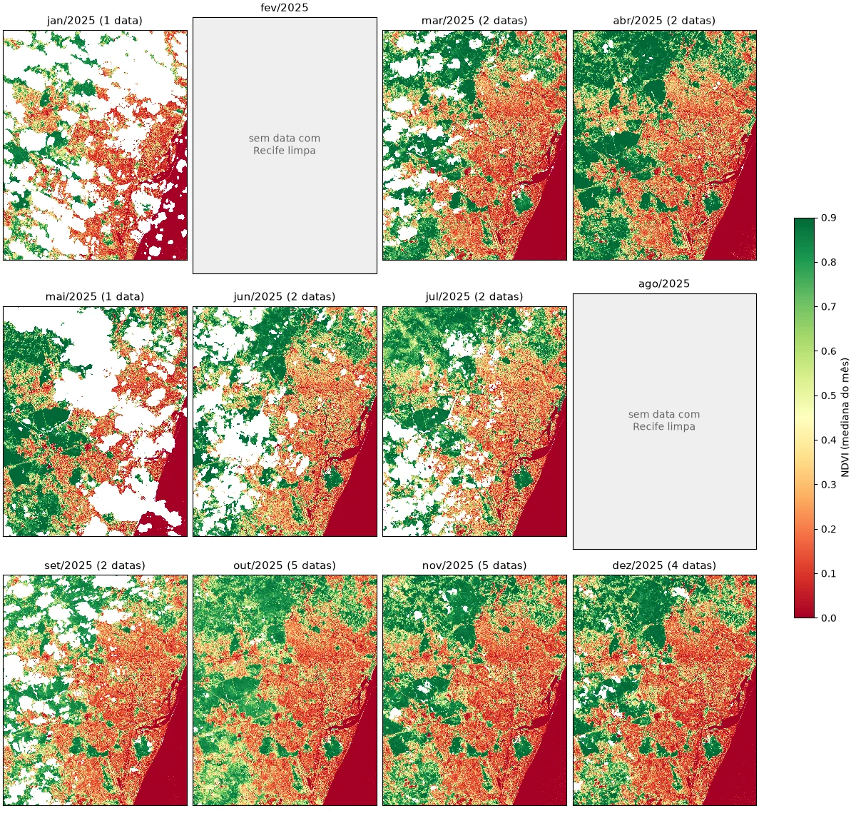
In the panel, the urban area shows up in orange and red, the forests to the west and north in dark green, and the sea and the Capibaribe river below zero. February and August have no date with at least half of Recife clear and were left empty. January and May depend on a single date and still have large cloud holes (in white). What partial reading changes is the cost of finding this out. Screening the year took seconds and the cube a few minutes, without downloading any scene.

Storing the result in Zarr and COG

The monthly NDVI is the product other analyses will consume, so it is worth storing it in a format that keeps the advantage of partial reading. We write the cube to Zarr, with one chunk per month and blocks of 512 × 512 pixels.

ds = ndvi_mensal.astype("float32").to_dataset(name="ndvi")
ds.chunk({"time": 1, "y": 512, "x": 512}).to_zarr("saida/ndvi_recife_2025.zarr", mode="w")

To extract the NDVI series of a dense forest point in the Dois Irmãos area, Zarr only needs to open the chunks that contain that pixel, one per month.

ds = xr.open_zarr("saida/ndvi_recife_2025.zarr")
x, y = Transformer.from_crs("EPSG:4326", "EPSG:32725", always_xy=True).transform(-34.936, -8.024)
serie = ds["ndvi"].sel(x=x, y=y, method="nearest").values

ndvi: (12, 2221, 1776) float32 | chunks de (1, 512, 512)
200 arquivos de chunk, 111.9 MB no disco (sem compressão seriam 180.6 MB)

ponto (-34.936, -8.024): chunks lidos 12 de 240
2025-01 nan
2025-02 nan
2025-03 0.903
2025-04 0.922
2025-05 nan
2025-06 0.911
2025-07 0.932
2025-08 nan
2025-09 0.892
2025-10 0.869
2025-11 0.875
2025-12 0.813

The cube has 240 possible chunks (12 months × 5 × 4 blocks), but only 200 became files. The 40 for February and August, entirely empty, were not even written, because Zarr 3 does not write chunks that contain only the fill value. With the default compression, the array's 180.6 MB take up 111.9 MB. For the point's series, 12 of the 240 chunks were read, 5% of the cube. If this Zarr were in a cloud bucket, that would be 12 small requests, not a download of the cube. The series shows the clouds again, with four months without an observation at this forest pixel, which sits between 0.81 and 0.93 when it shows up.

When the consumer is a GIS (QGIS, ArcGIS Pro) or a map server, the most practical format is COG. With GDAL 3.1 or newer, rioxarray writes directly with the COG driver.

outubro = ds["ndvi"].sel(time="2025-10").squeeze("time", drop=True)
outubro.rio.write_crs("EPSG:32725").rio.to_raster(
    "saida/ndvi_recife_2025_10.tif", driver="COG", compress="DEFLATE", predictor=3, blocksize=512
)

COG de outubro: {'px': [1776, 2221], 'bloco': [512, 512], 'overviews': [2, 4, 8], 'compressao': 'deflate', 'mb': 15.97, 'layout': 'COG'}

The file is 15.97 MB, with 512 × 512 blocks and three overview levels generated automatically. layout: COG confirms that GDAL wrote it in the optimized layout, with the index at the beginning of the file.

In day-to-day work, I use COG for one image per date, to be opened in a GIS or served as a map, and Zarr for a cube that code will slice in time and space.

The same code on another catalog

STAC's promise is that the same code works on any catalog. I tested the cloud-filtered search on Element 84's Earth Search, which indexes the copy of Sentinel-2 hosted on AWS.

CATALOGOS = {
    "Planetary Computer": ("https://planetarycomputer.microsoft.com/api/stac/v1", "sentinel-2-l2a"),
    "Earth Search": ("https://earth-search.aws.element84.com/v1", "sentinel-2-c1-l2a"),
}
for nome, (url, colecao) in CATALOGOS.items():
    itens = pystac_client.Client.open(url).search(
        collections=[colecao], bbox=BBOX, datetime="2025-01-01/2025-12-31",
        query={"eo:cloud_cover": {"lt": 20}},
    ).item_collection()
    datas = sorted({i.datetime.date().isoformat() for i in itens})
    print(f"{nome}: {len(itens)} itens, {len(datas)} datas, coleção {colecao}")
    print("  bandas do primeiro item:", ", ".join(sorted(itens[0].assets)[:12]), "...")

Planetary Computer: 7 itens, 5 datas, coleção sentinel-2-l2a
  bandas do primeiro item: AOT, B01, B02, B03, B04, B05, B06, B07, B08, B09, B11, B12 ...
Earth Search: 7 itens, 5 datas, coleção sentinel-2-c1-l2a
  bandas do primeiro item: aot, blue, cloud, coastal, granule_metadata, green, nir, nir08, nir09, preview, product_metadata, red ...

The search is identical and both catalogs return the same 5 dates, with none appearing in only one of them. But portability has limits that show up right at the next step. The asset names change (red and nir on Earth Search, B04 and B08 on Planetary Computer). And the sentinel-2-c1-l2a collection declares the scale and offset in the asset itself (scale: 0.0001, offset: -0.1 in raster:bands), which on Planetary Computer we apply by hand. STAC standardizes search and description, not the semantics of each collection. Switching catalogs means changing the URL, the collection name, a small band dictionary and checking the radiometry.

Final thoughts

We started from a year of imagery over Recife, 202 items in the catalog, and ended with a monthly NDVI stored in Zarr and COG without downloading any full scene. STAC found the scenes, the SCL read through the overviews picked out the useful dates in seconds and COG delivered only the city's blocks. The full files of the bands used would add up to 27.11 GB; the final product, in Zarr, is 111.9 MB.

This path pays off when the area of interest is much smaller than the scene, when the series has many dates and when processing can run close to the data, on a machine in the same cloud region. It loses strength when you will process full scenes over and over (then downloading once and working locally is cheaper) or when the connection is unstable, because every read depends on the network. And catalogs change with reprocessing, so for a reproducible study, keep the list of items used, as I did in the repository.

The data, the STAC items from the search and the programs in this article are in the blog repository on GitHub.

In the end, the habit changes more than the tool. The question stops being "which files do I need to download" and becomes "which bytes do I need to read".

References

• STAC Specification 1.1.0, Radiant Earth Foundation.
• Cloud Optimized GeoTIFF and GDAL COG driver.
• Zarr, specification and Python library.
• Microsoft Planetary Computer and Earth Search.
• odc-stac, loading STAC items into xarray.