Leak-free validation in time series: a Sentinel-2 soybean pixel, sequential evaluation and a sealed test

Translated from the original Portuguese article. Ler o original em português
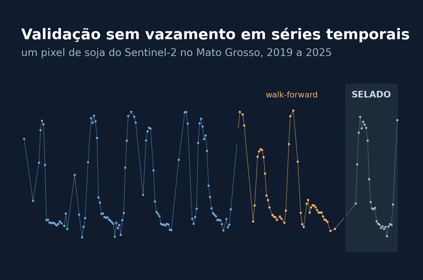
When I set up the evaluation protocol for a forecast on satellite image series, the first rule I write is not about the model. It is about when I am allowed to look at the test. It sounds excessive, but in time series it is very easy to build an evaluation that measures the model's ability to peek at the future, not to predict it.
The problem is that this kind of error does not break anything. The code runs, the metric looks great and the chart is convincing. The error only shows up when the model goes into production and starts receiving, each day, only what has already happened. Satellite imagery adds an aggravating factor, clouds. The series arrives full of holes, and the most common way to fill them uses, without anyone noticing, observations from the future.
In this article, I share the path I use to evaluate forecasts without data leakage: sequential evaluation (walk-forward), a period reserved for the final test and a metric that lets us compare models with a simple reference. The experiment uses real data from a single Sentinel-2 pixel inside a soybean field in Mato Grosso, Brazil, from 2019 to 2025. Training goes up to 2022, validation uses 2023 and 2024, and the test stays in 2025. Training fits the model; validation compares the alternatives and picks which one to use; the test measures the performance of that choice in a later period.
I use a Random Forest (RF), a model that combines several decision trees to produce the forecast. The configuration is simple on purpose, because the subject here is how to evaluate. As we will see, a leaky evaluation can artificially improve the score and even flip the decision about which model to use.
Searching for the images in the STAC catalog
I picked a point in a farming area of Mato Grosso, at (-13.3752, -54.4755). Each pixel is an image cell that represents a small area on the ground. Before using this point, I checked it in MapBiomas (the Brazilian annual land use and land cover mapping). The pixel is soybean (class 39) in 2017 and in 2023, and so is the whole 7×7 window of 30 m pixels around it. This position inside the area classified as soybean reduces the risk of mixing with roads or the field's edge. The MapBiomas rasters available for this check are only from those two years, so I did not verify the others; the curve of the normalized difference vegetation index (NDVI), in figure 1, helps examine the growing calendar, but does not confirm on its own the crop of each year.
The series comes from the Planetary Computer catalog, through the sentinel-2-l2a collection, of Sentinel-2 level 2A products. The catalog follows the STAC standard (SpatioTemporal Asset Catalog), which lets us find images by area, date and other metadata. Since we want a single pixel, we read only the region we need from each band. This is possible because the files are in COG (Cloud Optimized GeoTIFF), a format that lets us fetch parts of the image without transferring the whole file. That is about 1,800 small requests, three per scene.
from concurrent.futures import ThreadPoolExecutor

import pandas as pd
import numpy as np
import planetary_computer
import pystac_client
import rasterio
from rasterio.warp import transform
from sklearn.ensemble import RandomForestRegressor
from sklearn.model_selection import KFold

LAT, LON = -13.375151012548173, -54.47550071228342   # talhão de soja no MT (MapBiomas classe 39)

catalog = pystac_client.Client.open(
    "https://planetarycomputer.microsoft.com/api/stac/v1",
    modifier=planetary_computer.sign_inplace,
)
items = list(catalog.search(
    collections=["sentinel-2-l2a"],
    intersects={"type": "Point", "coordinates": [LON, LAT]},
    datetime="2019-01-01/2025-12-31",
).items())
print("cenas encontradas:", len(items))


def read_pixel(item):
    out = {"data": item.datetime.date(), "tile": item.properties["s2:mgrs_tile"],
           "baseline": item.properties.get("s2:processing_baseline")}
    for band in ["B04", "B08", "SCL"]:
        with rasterio.open(item.assets[band].href) as src:
            xs, ys = transform("EPSG:4326", src.crs, [LON], [LAT])
            r, c = src.index(xs[0], ys[0])
            out[band] = int(src.read(1, window=((r, r + 1), (c, c + 1)))[0, 0])
    return out


with ThreadPoolExecutor(16) as pool:
    rows = list(pool.map(read_pixel, items))
pd.DataFrame(rows).sort_values("data").to_csv("pixel_soja_s2.csv", index=False)
cenas encontradas: 597
The 597 scenes all belong to the same reference tile, identified as 21LYF, and the transfer took about five minutes on my machine. We keep B04 (red), B08 (near infrared) and the scene classification layer (SCL, Scene Classification Layer), which tells whether the pixel is vegetation, soil, cloud or shadow. The data, the cube and the programs in this article are in the blog repository on GitHub.
Computing NDVI: radiometric correction, cloud mask and repeated scenes
Before computing NDVI, there are three precautions. First, some dates appear twice because of reprocessing; we keep the most recent processing version, identified in the data as baseline. Second, we need to convert the digital number (DN), the integer value stored in each band, to the scale used in the computation. In the files of this experiment, we apply DN/10,000 before version 04.00 and (DN − 1,000)/10,000 from it onward. The subtraction of 1,000 corrects the additive offset introduced in these products. This rule depends on the source and on how the files were published, so it has to be checked when switching data. Third, we apply a quality mask and only accept the pixel when the SCL indicates vegetation (4) or bare soil (5).
To check this conversion, I compared one scene from each of the seven processing versions present in the file. In bands B04 and B08, the COGs' digital numbers matched the archived values. The XML files, which organize the products' metadata, confirmed the quantification factor of 10,000 and the offsets used. The COGs consulted indicated scale 1 and offset 0 on read; therefore, the conversion was applied after reading the digital numbers. This is a sample check, not a validation of every scene. The radiometric report records the items and the addresses of the official metadata.
df = pd.read_csv("pixel_soja_s2.csv", parse_dates=["data"])
df["baseline"] = pd.to_numeric(df["baseline"], errors="raise")
if not np.isfinite(df["baseline"]).all():
    raise ValueError("Baseline ausente ou inválida; confira os metadados antes de aplicar o offset.")
df = df.sort_values(["data", "baseline"]).drop_duplicates("data", keep="last")  # cena reprocessada: fica a mais nova
offset = np.where(df["baseline"] >= 4.0, 1000, 0)    # política radiométrica dos arquivos deste experimento
red = (df["B04"] - offset) / 10_000
nir = (df["B08"] - offset) / 10_000
df["ndvi"] = (nir - red) / (nir + red)
clean = df[df["SCL"].isin([4, 5])].set_index("data")["ndvi"]   # SCL 4 = vegetação, 5 = solo exposto
df_dev = df[df["data"] < pd.Timestamp("2025-01-01")]
clean_dev = clean[clean.index < pd.Timestamp("2025-01-01")]
print(f"até 2024: cenas {len(df_dev)} | limpas no pixel {len(clean_dev)}")
print("limpas por mês até 2024:", clean_dev.groupby(clean_dev.index.month).size().to_dict())
até 2024: cenas 421 | limpas no pixel 238
limpas por mês até 2024: {1: 11, 2: 8, 3: 11, 4: 22, 5: 25, 6: 33, 7: 34, 8: 34, 9: 26, 10: 16, 11: 11, 12: 7}
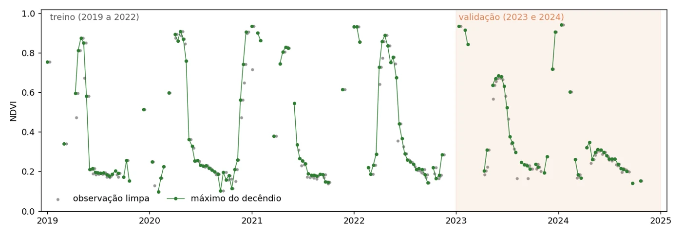
The curve shows NDVI rising from October and November, reaching close to 0.9 between December and January and falling in February. This pattern is consistent with the crop calendar assumed for the point. In most years, another growth cycle appears between March and June and, in the dry season, NDVI stays around 0.2. This second cycle changes from year to year, and in 2024 it barely shows up. The curve describes the observed vegetation, without identifying on its own the crop of each cycle.
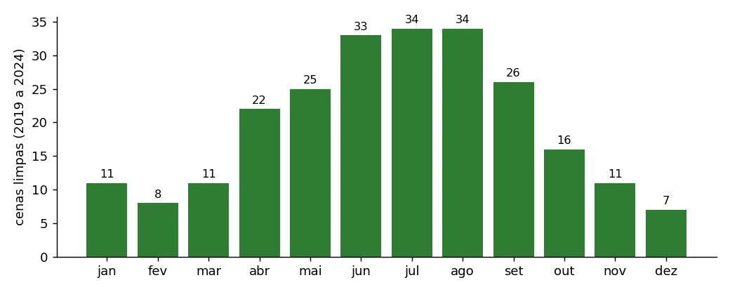
But figure 2 shows the problem that will guide the rest of the article. Clear observations are scarcest precisely during the growing season. From 2019 to 2024, December had 7 cloud-free scenes, against 34 in July. The forecast matters most when we see the crop least. Both this count and figure 1 use only the period before the test.
Dekadal series and the split into training, validation and test
To organize the series into regular intervals, we group the observations into dekads, ten-day periods (days 1 to 10, 11 to 20 and 21 to the end of the month). In each interval, we keep the highest NDVI among the observations accepted by the quality mask. This operation is the maximum value composite. There are 36 dekads per year, and a dekad with no valid scene stays empty.
def dekad(ts):
    return pd.Timestamp(ts.year, ts.month, 1 if ts.day <= 10 else 11 if ts.day <= 20 else 21)


grid = pd.DatetimeIndex([pd.Timestamp(y, m, d) for y in range(2019, 2026)
                         for m in range(1, 13) for d in (1, 11, 21)])
ndvi = clean.groupby(clean.index.map(dekad)).max().reindex(grid)   # máximo limpo do decêndio
TRAIN_END = ndvi.index.get_loc(pd.Timestamp("2023-01-01"))    # treino: 2019 a 2022
VAL_END = ndvi.index.get_loc(pd.Timestamp("2025-01-01"))      # validação: 2023 e 2024 | teste selado: 2025
dev = ndvi.iloc[:VAL_END].copy()                            # única série usada no desenvolvimento
gaps = dev.isna().astype(int)
longest = gaps.groupby((gaps != gaps.shift()).cumsum()).sum().max()
print(f"desenvolvimento: decêndios {len(dev)} | observados {dev.notna().sum()} | maior lacuna {longest}")
desenvolvimento: decêndios 216 | observados 150 | maior lacuna 6
In development, 66 of the 216 dekads are empty, and the longest gap lasts six dekads, about two months without a valid observation. All input tables, fits and comparisons used to select the model receive only the series up to 2024. This includes the leaky protocols we will build on purpose. That way, we can demonstrate the improper use of validation information without mixing it with the final test.
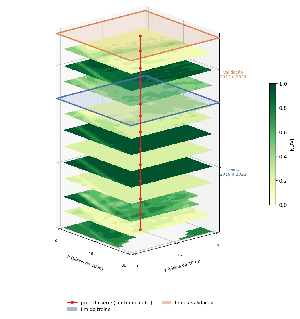
To see the pixel in context, I also extracted a 32×32 window of 10 m pixels (320 m per side) centered on the point and built the dekadal NDVI for each pixel. The result is a data cube, a sequence of images organized in two spatial dimensions and one temporal dimension. Figure 3 shows only 2019 to 2024. Each layer is a dekad, and the colored planes mark the end of training and of validation. For readability, I drew 14 of the 216 dekads. The red line runs through the central pixel, which is the series in figure 1, and it is the only one we will forecast. In this same period, the correlations of the 1,024 pixels with the central one, computed on pairs of valid observations, have a median of 0.97; 61.6% are above 0.9. This agreement describes the chosen window, without enlarging the sample used to evaluate the forecasts.
The target, that is, the value we want to predict, is the maximum clear NDVI of the next dekad. The forecast is issued at the opening of that interval, assuming the previous dekad's composite is already available. We call that moment the forecast origin. The horizon is one step. We estimate the next dekad, an interval of about ten days. This does not mean exactly ten days of lead time for each image. The simulation does not include product publication delays or the historical availability of their reprocessed versions.
We call causal inputs the variables built only with information prior to the forecast origin. In this article, the term "causal" describes this temporal availability. It is the rule that lets us build an input as it would be available at the moment the model is used.
There is one more important decision: error is measured only where there is a real observation. Evaluating against interpolated values would confuse the quality of the forecast with that of the gap filling. On the other hand, the error in fully overcast dekads is not directly verifiable in this experiment. The metrics describe performance over the periods with an observed target.
MASE with persistence as the reference
Before measuring any model, we need a reference to interpret the error. We use an adaptation of the Mean Absolute Scaled Error (MASE), proposed by Hyndman and Koehler, 2006. The adaptation accounts for irregular observability, since persistence repeats the last available observation, which may be older than the previous dekad.
The definition used here is adapted MASE = mean absolute error on the evaluation's observed targets / mean absolute error of persistence in training. The Mean Absolute Error (MAE) is the average distance between predicted and observed values, ignoring the sign of the differences. The denominator considers only training instants with both a target and a persistence forecast available, and it stays fixed across comparisons. MASE below 1 means erring less than persistence did in training. To know whether a model beats persistence in validation or test, we compare the two over the same period.
LAGS = (1, 2, 3)


def eligible_rows(series, end):
    return [i for i in range(max(LAGS) + 1, end) if pd.notna(series.iloc[i])]


def fill(series):
    """Preenche lacunas: interpola entre observações e repete a última no fim."""
    return series.interpolate(limit_area="inside").ffill()


def persistence(series, start, end):
    """Previsão ingênua: o último NDVI conhecido antes de cada decêndio."""
    return pd.Series([fill(series.iloc[:o]).iloc[-1] for o in range(start, end)],
                     index=series.index[start:end])


SCALE = (dev.iloc[1:TRAIN_END] - persistence(dev, 1, TRAIN_END)).abs().mean()


def mase(y_true, y_pred):
    """MAE só onde há observação real, dividido pelo MAE da persistência no treino."""
    ok = y_true.notna()
    if not y_true.index.equals(y_pred.index) or not np.isfinite(y_pred[ok]).all():
        raise ValueError("É necessária uma previsão finita e alinhada para cada alvo observado.")
    return np.mean(np.abs(y_true[ok] - y_pred[ok])) / SCALE


val = dev.iloc[TRAIN_END:VAL_END]
pers_val = persistence(dev, TRAIN_END, VAL_END)
last_year = pd.Series([fill(dev.iloc[:o]).iloc[o - 36] for o in range(TRAIN_END, VAL_END)], index=val.index)
print(f"escala: {SCALE:.3f} de NDVI | decêndios avaliados na validação: {val.notna().sum()}")
print(f"persistência: MASE = {mase(val, pers_val):.3f}")
print(f"mesmo decêndio do ano anterior: MASE = {mase(val, last_year):.3f}")
escala: 0.101 de NDVI | decêndios avaliados na validação: 46
persistência: MASE = 0.952
mesmo decêndio do ano anterior: MASE = 1.738
Persistence errs, on average, by 0.101 NDVI per dekad in training, and, in validation, its MASE is 0.952. Repeating the same dekad from the previous year is much worse (1.738). It makes sense, because the planting date varies by a few weeks from one year to the next and the second crop does not always exist, so "last year" errs precisely on the rises and falls of the curve. That is why persistence stays as the reference any model has to beat to justify the extra complexity.
Cross-validation with five random folds
Now we build the supervised learning table, in which each example associates input variables with a known target. Each row corresponds to a dekad t. The input variables (features) are the NDVI of the three previous dekads, with gaps filled, and the dekad's position in the year. These previous values are the lags of one, two and three steps. The target is the NDVI observed in dekad t.
def make_features(series):
    """Linha do decêndio t: NDVI preenchido nos 3 decêndios anteriores e o decêndio do ano."""
    f = fill(series)
    X = pd.DataFrame({f"lag_{k}": f.shift(k) for k in LAGS})
    X["dekad_of_year"] = (series.index.month - 1) * 3 + (series.index.day - 1) // 10
    return X


def new_model(seed=42):
    return RandomForestRegressor(n_estimators=300, min_samples_leaf=3, random_state=seed, n_jobs=-1)
We start with the deliberately wrong protocol. We fill the whole development period, build the table and apply KFold, the implementation of k-fold cross-validation. We use five groups, called folds. In each round, four train the model and the remaining one is used to evaluate it. Rows are shuffled without respecting time order. So a forecast can be evaluated by a model trained on later observations. To compare protocols, we measure the error on the same 46 observed validation dekads and keep the folds to reuse them in the causal input condition.
X_all = make_features(dev)                             # interpolação global só até 2024
dev_rows = eligible_rows(dev, VAL_END)
X_dev, y_dev = X_all.iloc[dev_rows], dev.iloc[dev_rows]
folds = list(KFold(n_splits=5, shuffle=True, random_state=42).split(X_dev))
pred_kf = pd.Series(index=y_dev.index, dtype=float)
for tr, te in folds:
    pred_kf.iloc[te] = new_model().fit(X_dev.iloc[tr], y_dev.iloc[tr]).predict(X_dev.iloc[te])
pred_kf = pred_kf.reindex(val.index)
print(f"KFold aleatório: MASE = {mase(val, pred_kf):.3f}")
KFold aleatório: MASE = 0.578
Comparing 0.578 with persistence's 0.952 on the same validation, the Random Forest seems to err 39.3% less. That would be a great result for a series with so much cloud. But this evaluation mixes two problems, since the folds include training on later observations and the lags come from interpolating the whole development period. Further on, we compare the combinations to understand how each choice relates to the result.
Interpolating the gaps before the split
Replacing the shuffle with time order seems enough: we train on 2019 to 2022 and predict 2023 and 2024 in order. But if the gaps were filled over the whole series before the split, the leak is still there, only hidden.
train_rows = eligible_rows(dev, TRAIN_END)
model = new_model().fit(X_all.iloc[train_rows], dev.iloc[train_rows])
pred_pre = pd.Series(model.predict(X_all.iloc[TRAIN_END:VAL_END]), index=val.index)
print(f"walk-forward, lacunas preenchidas antes: MASE = {mase(val, pred_pre):.3f}")
walk-forward, lacunas preenchidas antes: MASE = 0.887
The model still seems 6.8% better than persistence, and figure 4 shows where that gain comes from. On 02/11/2024 we want to predict an NDVI that, as we learn later, was 0.602. The two previous dekads were covered by clouds. Interpolation done over the whole series fills them with 0.829 and 0.715, a line already heading down toward the target, because it was drawn using the target itself. Someone in the field on 02/11 would only know that the last clear image, from the 01/11 dekad, read 0.942.
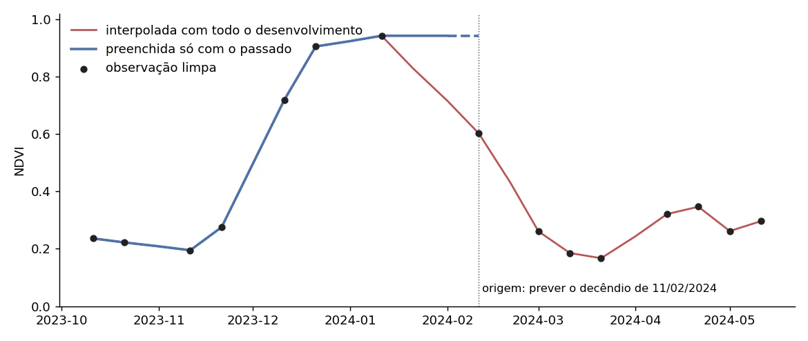
In linear interpolation, missing values are filled with a line between two known observations. If the observation on the right is not yet available at the forecast origin, it transfers information from the future into the input. The same care applies to smoothing, such as Savitzky-Golay and Whittaker filters, when applied using observations on both sides in time. In satellite image series, this preprocessing may sit in a separate program, run before modeling, which makes the leak harder to notice.
Sequential evaluation with training and forecasting using only the past
Sequential evaluation (walk-forward) goes through the dekads in order and simulates a forecast at each origin. Here, the model is fit once before validation. Its parameters stay fixed, while the inputs incorporate the new observations already available. At each origin o, the input row is recomputed using only the series up to o - 1, with the value at o left blank.
def row_for_day(series, o, features=make_features):
    """A linha do decêndio o montada só com o passado: o valor de o fica vazio."""
    past = series.iloc[:o]
    blank = pd.Series([np.nan], index=series.index[o:o + 1])
    return features(pd.concat([past, blank])).iloc[[-1]]


def walk_forward(series, start, end, features=make_features, past_only_train=True):
    """Ajusta uma vez antes de start e prevê cada decêndio de [start, end) só com o passado."""
    rows = eligible_rows(series, start)
    if past_only_train:    # cada linha de treino montada como seria no dia dela
        X_tr = pd.concat([row_for_day(series, i, features) for i in rows])
    else:                  # linhas de treino da série de treino preenchida de uma vez
        X_tr = features(series.iloc[:start]).iloc[rows]
    model = new_model().fit(X_tr, series.iloc[rows])
    preds = [model.predict(row_for_day(series, o, features))[0] for o in range(start, end)]
    return pd.Series(preds, index=series.index[start:end])


pred_mix = walk_forward(dev, TRAIN_END, VAL_END, past_only_train=False)
pred_wf = walk_forward(dev, TRAIN_END, VAL_END)
print(f"walk-forward, só a previsão com o passado: MASE = {mase(val, pred_mix):.3f}")
print(f"walk-forward, treino e previsão com o passado: MASE = {mase(val, pred_wf):.3f}")
walk-forward, só a previsão com o passado: MASE = 1.243
walk-forward, treino e previsão com o passado: MASE = 1.148
The past_only_train parameter lets us compare two ways of building the training inputs. When it is false, only the forecast inputs respect each origin; the training rows come from the training series filled all at once. In that case, the training lags may incorporate information later than the instant they represent, while the inputs at use time depend only on the past. This mismatch between training and use (training-serving skew) yields a MASE of 1.243. Building the training rows too as they would be available on the day of each forecast brings MASE to 1.148. Both conditions are part of the comparison between protocols.
The row_for_day function builds the input row of an origin using only the past. With it, we repeat the same random KFold, keeping the folds and changing how each row is built:
X_dev_p = pd.concat([row_for_day(dev, i) for i in dev_rows])   # mesmas linhas, entradas causais
y_dev_p = y_dev
pred_kf_p = pd.Series(index=y_dev_p.index, dtype=float)
for tr, te in folds:                                       # mesmas dobras da versão interpolada
    pred_kf_p.iloc[te] = new_model().fit(X_dev_p.iloc[tr], y_dev_p.iloc[tr]).predict(X_dev_p.iloc[te])
pred_kf_p = pred_kf_p.reindex(val.index)
print(f"KFold aleatório, linhas só com o passado: MASE = {mase(val, pred_kf_p):.3f}")
KFold aleatório, linhas só com o passado: MASE = 1.118
The four combinations help read the result:
| Data split | Interpolation of the whole development period | Causal inputs per origin |
|---|---|---|
| Random KFold | 0.578 | 1.118 |
| Chronological, fixed model | 0.887 | 1.148 |
With causal inputs, KFold comes close to the chronological evaluation for this pixel. Global interpolation, on the other hand, is associated with the largest reductions in apparent error, especially when combined with shuffled folds. The comparisons point to this interpolation as the main source of the observed optimism, but they do not allow us to assign an exact share of the effect to each change, because the protocols also differ in the composition and period of training. The result holds for this pixel and these input variables. Random KFold remains inadequate to simulate future forecasting because it includes training on observations later than the evaluated target.
Back to the sequential evaluation, 1.148 is still 20.6% worse than persistence. In long gaps, the model does not know it is looking at an old image. So we give it that information, honest and available on the day, namely how many dekads ago the last clear observation came in. This is the age of the observation, measured in dekads.
def make_features_age(series):
    """As mesmas features e há quantos decêndios saiu a última observação limpa."""
    X = make_features(series)
    pos = np.arange(len(series))
    last_seen = pd.Series(np.where(series.notna(), pos, np.nan), index=series.index).ffill()
    X["obs_age"] = pos - last_seen.shift(1).to_numpy()
    return X


pred_age = walk_forward(dev, TRAIN_END, VAL_END, features=make_features_age)
print(f"walk-forward com idade da observação: MASE = {mase(val, pred_age):.3f}")
walk-forward com idade da observação: MASE = 1.070
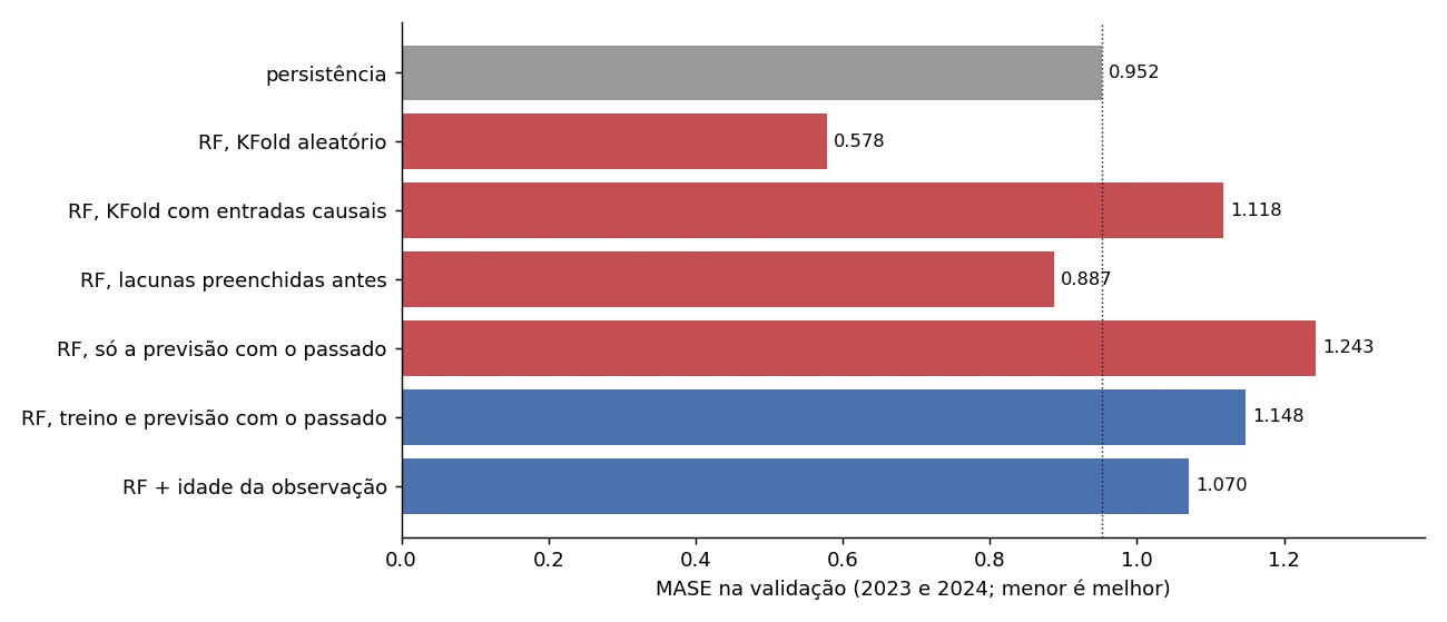
Figure 5 summarizes the validation. The red bars represent different problems: training on later observations in KFold, interpolation that uses observations before and after in the inputs, or building the training set with information that would not be available at each origin. These problems do not produce an apparent gain in every configuration. KFold with global interpolation and the prior filling stay below persistence; KFold with causal inputs and the condition that is causal only at forecast time stay above. In the first two cases, the comparison of mean errors suggests a model switch that the causal evaluation does not support. The uncertainty analysis shows how much we can conclude from these differences.
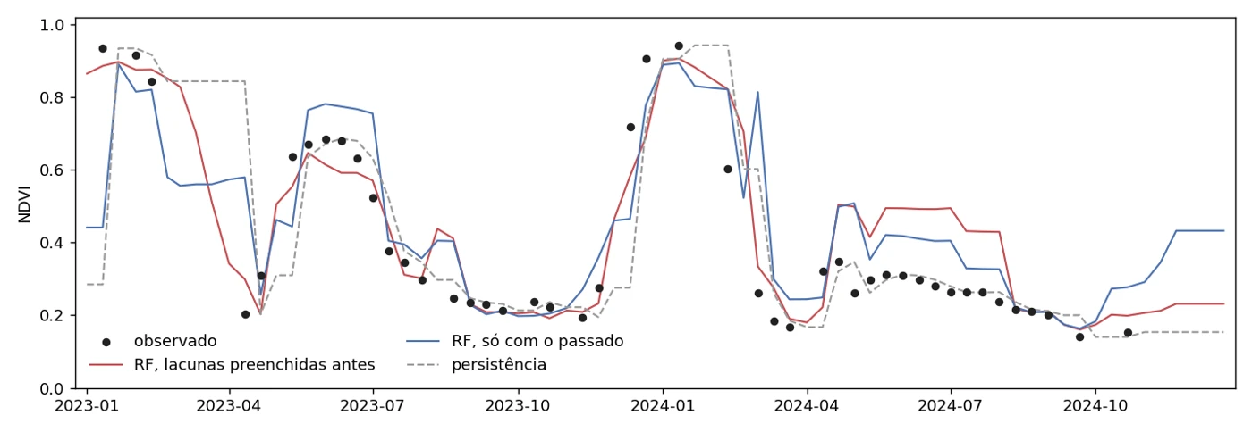
In figure 6, you can see where the honest model loses. After the 2023 harvest and in March 2024, it is slow to follow the NDVI drop, stuck on high values from old images, because the gap hides the harvest. The model with gaps filled beforehand looks smarter precisely in these stretches, because the interpolation already handed it the direction of the curve.
Error by crop phase: growing season and the rest of the year
The average hides an important split. Of the 46 observed validation dekads, only 12 fall in the soybean season, from October to February; the other 34 are in the rest of the year, when NDVI changes slowly. Splitting the error by the two phases:
safra = val.index.month.isin([10, 11, 12, 1, 2])
print(f"decêndios observados: safra {val[safra].notna().sum()} | resto do ano {val[~safra].notna().sum()}")
for name, p in [("persistência", pers_val), ("lacunas preenchidas antes", pred_pre),
                ("treino e previsão com o passado", pred_wf), ("RF + idade da observação", pred_age)]:
    print(f"{name}: safra {mase(val[safra], p[safra]):.3f} | resto do ano {mase(val[~safra], p[~safra]):.3f}")
decêndios observados: safra 12 | resto do ano 34
persistência: safra 1.572 | resto do ano 0.733
lacunas preenchidas antes: safra 0.735 | resto do ano 0.940
treino e previsão com o passado: safra 1.323 | resto do ano 1.086
RF + idade da observação: safra 1.243 | resto do ano 1.009
All honest models err more during the season, when the crop changes fast and the clouds hide the change. But in this phase, the honest Random Forest beats persistence (1.243 against 1.572, with the age of the observation). It loses in the rest of the year, when repeating the last image is nearly unbeatable (0.733). Since that period has almost three times as many points, it is the one that decides the average. The model with gaps filled beforehand reaches 0.735 precisely during the season, where the gaps are longest, which is consistent with the interpolation handing over more of the future exactly there.
How much of these differences is noise
So far, the results use seed 42 and 46 observed targets. The random seed is the number that initializes the random draws and lets us repeat a run under the same conditions. To examine the variation, I repeated the evaluations with seeds 0 to 9. In the Random Forest, the model's randomness changes; in KFold, the folds change too. Within each seed, the global interpolation and causal input conditions use exactly the same rows and folds. Therefore, this table measures the joint sensitivity to the model and, in the KFold protocols, to the data split. Seed 42 is not part of these ten repetitions.
| Evaluation on validation | minimum | median | maximum |
|---|---|---|---|
| Random KFold | 0.521 | 0.556 | 0.587 |
| gaps filled beforehand | 0.824 | 0.848 | 0.876 |
| Random KFold, rows using only the past | 0.984 | 1.077 | 1.111 |
| only the forecast using the past | 1.179 | 1.207 | 1.231 |
| training and forecast using the past | 1.123 | 1.144 | 1.160 |
| RF + observation age | 1.046 | 1.067 | 1.092 |
Across the ten seeds, KFold with global interpolation and the chronological protocol with prior filling stay below persistence's 0.952. The configurations with causal training and forecasting stay above. The other two protocols with methodological problems also stay above the reference, showing that leakage or a train-use mismatch do not guarantee a reduction in apparent error.
The seed, however, is not the only source of variation. To examine the uncertainty associated with the observed period, I used a block bootstrap. The procedure builds new samples by drawing stretches of the full time grid. The draw is with replacement, meaning the same stretch can appear more than once in the sample. In each repetition, we recompute the MASE difference between the model and persistence. Only after building the sample do we select the observed targets. That way, the blocks keep the local order and the gaps within each stretch, without treating the 46 targets as if they were necessarily consecutive. The computation keeps the forecasts and the training scale fixed, without refitting the models in each resample.
We start with blocks of six dekads, about two months, and 5,000 resamples. In the outputs, IC95% (the Portuguese abbreviation) identifies the 95% confidence interval, computed here between the 2.5th and 97.5th percentiles of the resampled differences. These percentiles are the limits that leave 2.5% of the differences at each tail of the distribution. The last column reports the proportion of resamples with a negative difference (proporção negativa), favorable to the model. It is not a calibrated probability that the model is superior.
def block_bootstrap_diff(y_true, pred, ref, block=6, n=5000, seed=0):
    """IC percentil e proporção de reamostragens com diferença de MASE negativa."""
    if not 1 <= block <= len(y_true) or n < 1:
        raise ValueError("Bloco e número de reamostragens inválidos.")
    mase(y_true, pred)  # confere alinhamento e previsões nos alvos observados
    mase(y_true, ref)
    rng = np.random.default_rng(seed)
    ok = y_true.notna().to_numpy()
    e_m = np.abs(y_true - pred).to_numpy() / SCALE
    e_r = np.abs(y_true - ref).to_numpy() / SCALE
    T = len(y_true)
    starts = np.arange(T - block + 1)
    diffs = []
    for _ in range(n):
        idx = np.concatenate([np.arange(s, s + block) for s in rng.choice(starts, size=int(np.ceil(T / block)))])[:T]
        sel = idx[ok[idx]]
        if len(sel) == 0:
            continue
        diffs.append(e_m[sel].mean() - e_r[sel].mean())
    if not diffs:
        raise ValueError("Nenhuma reamostragem continha um alvo observado.")
    diffs = np.array(diffs)
    point = e_m[ok].mean() - e_r[ok].mean()
    return point, np.percentile(diffs, 2.5), np.percentile(diffs, 97.5), (diffs < 0).mean()


for name, p in [("KFold aleatório", pred_kf), ("KFold só com o passado", pred_kf_p),
                ("lacunas preenchidas antes", pred_pre), ("treino e previsão com o passado", pred_wf),
                ("RF + idade", pred_age)]:
    d, lo, hi, p_neg = block_bootstrap_diff(val, p, pers_val)
    print(f"{name}: {d:+.3f}  IC95% [{lo:+.3f}; {hi:+.3f}]  proporção negativa = {p_neg:.2f}")
KFold aleatório: -0.374  IC95% [-0.717; -0.017]  proporção negativa = 0.98
KFold só com o passado: +0.166  IC95% [-0.108; +0.440]  proporção negativa = 0.12
lacunas preenchidas antes: -0.065  IC95% [-0.631; +0.600]  proporção negativa = 0.49
treino e previsão com o passado: +0.196  IC95% [-0.129; +0.492]  proporção negativa = 0.11
RF + idade: +0.118  IC95% [-0.214; +0.433]  proporção negativa = 0.20
With blocks of six dekads, only KFold with global interpolation has an interval entirely below zero. In the two evaluations with causal training and forecasting, the intervals include zero, and the Random Forest comes out ahead of persistence in about 11% to 20% of the resamples. This does not show that the models are equivalent or that the Random Forest is necessarily worse; this validation shows no clear evidence of a gain.
To check how much the reading depends on block size, I repeated the computation with three and twelve dekads. The table shows the 95% percentile intervals of the MASE difference, always model minus persistence:
| Evaluation | Blocks of 3 | Blocks of 6 | Blocks of 12 |
|---|---|---|---|
| KFold with global interpolation | [-0.727; -0.030] | [-0.717; -0.017] | [-0.711; +0.001] |
| KFold with causal inputs | [-0.074; +0.415] | [-0.108; +0.440] | [-0.123; +0.461] |
| Gaps filled beforehand | [-0.576; +0.482] | [-0.631; +0.600] | [-0.689; +0.708] |
| Training and forecast using the past | [-0.103; +0.479] | [-0.129; +0.492] | [-0.143; +0.532] |
| RF + observation age | [-0.197; +0.415] | [-0.214; +0.433] | [-0.259; +0.473] |
The absence of a clear gain in the causal evaluations holds for all three choices. The interval of KFold with global interpolation, however, starts to include zero with blocks of twelve dekads. Its advantage in the point estimate, computed on the observed data, remains, but the statement about the interval depends on the choice of block. Two years of validation also limit the examination of longer seasonal dependencies. The full results are in the block bootstrap table and in the run reproduction record, which reports the library versions, the settings and the identifiers of the files used.
Hey João, so the Random Forest is no good for this?
That is not what the experiment says. It says that, with these inputs, on a single pixel and with 46 observed targets in validation, we did not demonstrate a gain that justifies replacing persistence. Other pixels and other variables may change the result, but they require new experiments. Without the causal evaluation, the apparent 39.3% reduction in error could support a choice the available results do not justify.
Final evaluation on the 2025 test
The decision rule is simple: the more complex model only replaces persistence if it has a lower mean error in validation; the uncertainty analysis helps qualify that comparison. The Random Forest with causal inputs does not beat the reference on average in any of the ten seeds, so the choice is persistence. This selection happens before computing the 2025 results.
The test is called "sealed" because it stays outside the input building, fitting and comparison steps used to select the model. The figures and exploratory statistics use only data up to 2024. After the selection, we compute the performance in 2025; additional comparisons in that period are descriptive and do not redefine the choice. The evaluation is a simulation on historical data, with the observation availability assumptions described in the protocol.
sealed = ndvi.iloc[VAL_END:]
pers_test = persistence(ndvi, VAL_END, len(ndvi))
print(f"decêndios avaliados no teste: {sealed.notna().sum()}")
print(f"teste selado, persistência: MASE = {mase(sealed, pers_test):.3f}")
decêndios avaliados no teste: 27
teste selado, persistência: MASE = 0.910
Persistence scores 0.910 in 2025, close to the 0.952 from validation. This is the number that goes into the report.
As a descriptive comparison, we also evaluate the Random Forest with the age of the observation. In this step, it is fit on data from 2019 to 2024, keeping the same causal inputs and settings. During 2025, its parameters stay fixed and the inputs receive only observations prior to each forecast. The MASE scale is still the one computed in the training period, 2019 to 2022.
pred_test_age = walk_forward(ndvi, VAL_END, len(ndvi), features=make_features_age)
print(f"teste selado, RF + idade da observação: MASE = {mase(sealed, pred_test_age):.3f}")
teste selado, RF + idade da observação: MASE = 0.874
In 2025, the Random Forest was 4.0% better than persistence, the opposite of what validation showed. Running the test through the same bootstrap:
d, lo, hi, p_neg = block_bootstrap_diff(sealed, pred_test_age, pers_test)
print(f"RF + idade (teste): {d:+.3f}  IC95% [{lo:+.3f}; {hi:+.3f}]  proporção negativa = {p_neg:.2f}")
RF + idade (teste): -0.036 IC95% [-0.262; +0.219] proporção negativa = 0.50
Hey João, so should I switch to the Random Forest?
Not based on this comparison. Switching now would use the 2025 result to select the model. With blocks of six dekads, the interval of the difference goes from -0.262 to +0.219 and includes zero. The same happens with blocks of three, whose interval is [-0.333; +0.304], and of twelve, [-0.156; +0.139]. Across the ten seeds, the Random Forest's point estimate stays below 0.910, but that stability does not remove the uncertainty of evaluating only 27 observed targets in one year. The available results do not demonstrate a clear gain. A new decision requires freezing the protocol and evaluating a future block not yet consulted.
Conclusion
We started with a Random Forest that, under KFold with global interpolation, seemed to err 39.3% less than persistence. In the comparison between protocols, interpolation is associated with most of the optimism observed for this pixel. Respecting time order but keeping the prior filling, the apparent advantage was still 6.8%. With causal training and forecasting, the mean error was 20.6% above persistence, or 12.4% with the age of the observation. The choice of persistence held across the ten seeds. The bootstrap with blocks of three, six and twelve dekads showed no clear evidence of a gain in the causal evaluations. In 2025, persistence scored 0.910, close to the 0.952 from validation; the Random Forest's small point advantage that year also came with intervals that include zero.
The protocol starts with the chronological split and with defining what is available at each origin. Training and forecast inputs must respect that availability, and models must be compared with a simple reference on the same set of targets. Steps that learn preprocessing parameters must also respect the training data allowed by the protocol. When following future forecasts in a prospective evaluation, the test must stay out of the decisions, with the choices recorded before it is opened. This discipline keeps the evaluation aligned with how the model will be used.
This is a demonstration study of one pixel, with 46 observed targets in validation and 27 in the test. The numbers show how the evaluation changes in this case; they do not estimate the typical magnitude of leakage in other regions, crops or cloud conditions. Nor do they establish the error in periods without a valid observation. Those extensions depend on independent experiments.
In satellite image series, this care weighs even more, because clouds are not just noise. They decide what the model can know in each dekad. For this pixel, it was during the growing season, the cloudiest phase, that interpolation most favored the leaky model and that all honest models erred the most. Validating without leakage means measuring the model by what it does with the sky it actually had, not with the clean curve we draw afterwards.
Reference
HYNDMAN, Rob J.; KOEHLER, Anne B. Another look at measures of forecast accuracy. International Journal of Forecasting, v. 22, n. 4, p. 679-688, 2006. DOI: 10.1016/j.ijforecast.2006.03.001