GetCompress: Compressing Raster Stacks to Run Faster Without Losing the Original Grid

I was reading the paper by Almaghrabi et al. (2024) on multivariate time series forecasting of solar power generation using multilevel data fusion. In the middle of the discussion, one practical idea kept nagging at me: in day-to-day work with large, heterogeneous data, the bottleneck is often not the model, but how we represent and move that data through the pipeline. That made me want to start writing here again and share a solution to a very common problem in geoprocessing: how to operate on giant rasters without wasting memory and I/O on empty areas.

When a raster goes into production, especially at national scale, the bottleneck is almost never a "lack of model". In practice, what weighs on us is volume, I/O and wasted memory. We need to load a huge grid to represent the entire territory, but a large part of it carries no useful information, such as sea, borders, nodata and resampling holes.

The idea behind GetCompress is simple: swap "processing a gigantic H×W full of emptiness" for "processing only what is occupied", while keeping a contract that allows us to rebuild the original grid whenever needed.

It is worth stressing that we are not talking about entropy-based compression here, such as LZW and DEFLATE. The focus is structural compression, that is, removing empty space and working only with valid pixels. In scenarios with a lot of nodata, the gain usually shows up immediately.

We start with the basics: we organize the imports, define an output NoData value and make an important choice, whether NaN should be treated as NoData. This decision about the output NoData seems small, but it avoids noise in production. NoData as NaN in a GeoTIFF can get in the way of tools and simple operations, while 0 tends to be more predictable when we publish a binary product, such as masks and thresholds.

import numpy as np
import rasterio
import json
from rasterio.transform import Affine

import matplotlib.pyplot as plt

NODATA_OUT = 0
TREAT_NAN_AS_NODATA = True

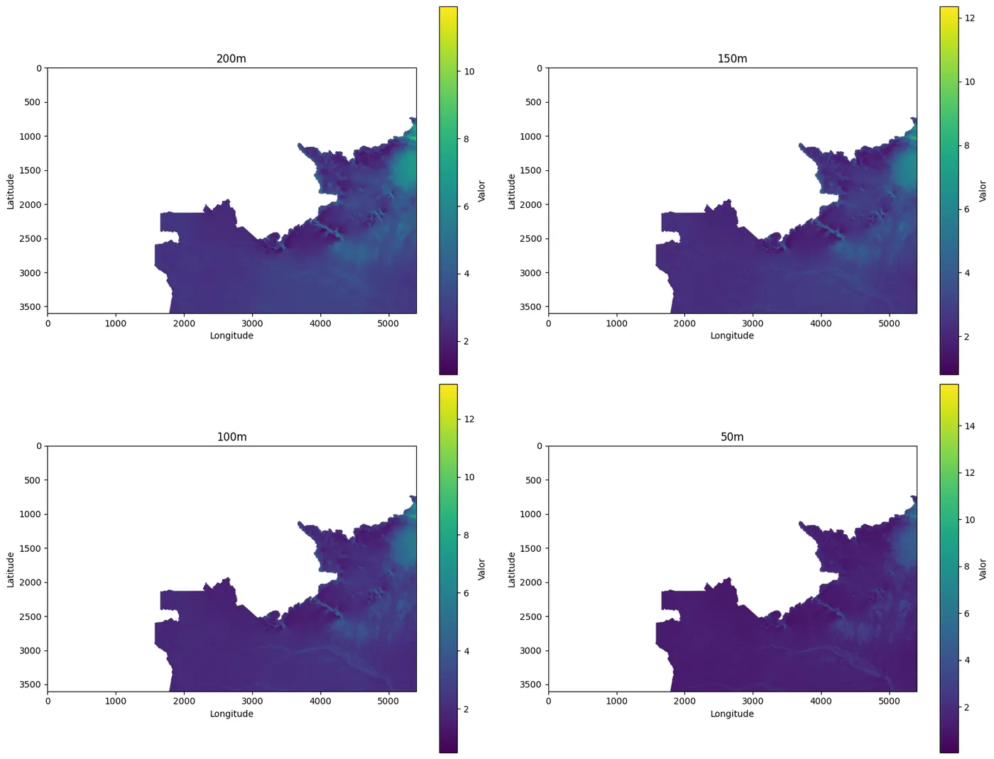
Before applying the compression, we make sure the stack is coherent and well aligned. A quick visual inspection at the start of the workflow usually saves rework when there is misalignment, truncation or unexpected NoData patterns. That is why we create two simple routines: one to display a 2D raster and another to display a stack, limiting the visualization to at most four bands to keep the check focused and fast.

With these functions, we now have a sanity check for the pipeline. If a shifted band, an entirely zeroed strip or an incorrect crop shows up, we fix the problem before generating the mask, packing and saving the artifacts.

def plot_raster(data, title='', cmap='viridis', figsize=(10, 8)):
    plt.figure(figsize=figsize)
    plt.imshow(data, cmap=cmap)
    plt.colorbar(label='Valor')
    plt.title(title)
    plt.xlabel('Longitude')
    plt.ylabel('Latitude')
    plt.tight_layout()
    plt.show()

def plot_stack(stack, titles=None, cmap='viridis', figsize=(16, 12)):
    if stack.ndim != 3:
        raise ValueError("Stack deve ter 3 dimensões (C, H, W)")

    n_bands = stack.shape[0]
    if titles is None:
        titles = [f'Banda {i+1}' for i in range(n_bands)]

    fig, axes = plt.subplots(2, 2, figsize=figsize)
    axes = axes.flatten()

    for i in range(min(n_bands, 4)):
        im = axes[i].imshow(stack[i], cmap=cmap)
        axes[i].set_title(titles[i])
        axes[i].set_xlabel('Longitude')
        axes[i].set_ylabel('Latitude')
        plt.colorbar(im, ax=axes[i], label='Valor')

    plt.tight_layout()
    plt.show()

What we call an occupied pixel

Now we define the rule that decides which pixels go into the packing. Here we use a pragmatic approach that suits multiband stacks: a pixel is considered occupied if at least one band has a valid value. This way we avoid losing useful information when one of the bands has isolated gaps.

To build the mask, we combine two notions of emptiness. The first is the presence of NaN, common in floating-point rasters. The second is an explicit NoData, when the file defines a sentinel value in its metadata. From there, we reduce the stack to a 2D mask by applying the criterion "there is at least one valid band". This guarantees that the selected set of pixels is unique and consistent across all bands, avoiding discrepancies between channels during processing.

def get_occupied_mask(stack, nodata, treat_nan_as_nodata=True):
    if stack.ndim != 3:
        raise ValueError("stack deve ser (C,H,W)")
    data = stack

    ok = np.ones_like(data, dtype=bool)

    if treat_nan_as_nodata and np.issubdtype(data.dtype, np.floating):
        ok &= np.isfinite(data)

    if nodata is not None:
        ok &= (data != nodata)

    return np.any(ok, axis=0)  # (H,W)

Dense packing and the reversal contract

With the mask in hand, we perform the structural compression. The goal is to pack the valid values into a nearly square dense grid and, at the same time, store a reversal contract that allows us to rebuild the original grid without ambiguity.

This contract is idx, a vector of linear indices into the original grid. In practice, it is the map that links the compressed domain back to the original spatial domain. With it, CPU and RAM cost becomes proportional to N, the number of occupied pixels, rather than to the H×W of the whole raster.

In the packing step, we start by extracting the indices where the mask is true and compute N, the number of valid pixels. Next, we define the width and height of the dense container, allocate an array filled with NoData and copy only the valid values into it, in row-major order. Finally, we record in the metadata all the information needed to reverse the compression and rebuild the original grid.

As a result, CPU and RAM cost grows in proportion to N rather than to the product H×W, avoiding unnecessary processing over large empty regions.

def compress_raster(stack, nodata, treat_nan_as_nodata=True):
    C, H, W = stack.shape
    mask = get_occupied_mask(stack, nodata, treat_nan_as_nodata)
    idx = np.flatnonzero(mask.ravel())  # índices lineares dos pixels válidos no original
    N = idx.size

    if N == 0:
        packed = np.full((C, 1, 1), nodata, dtype=stack.dtype)
        meta = dict(H=H, W=W, C=C, idx=idx, h=1, w=1, nodata=nodata)
        return packed, meta

    # tamanho da grade densa (quase quadrada)
    w_new = int(np.ceil(np.sqrt(N)))
    h_new = int(np.ceil(N / w_new))

    packed = np.full((C, h_new, w_new), nodata, dtype=stack.dtype)

    # extrai valores válidos (C,N) e coloca row-major
    vals = stack.reshape(C, -1)[:, idx]  # (C,N)
    packed.reshape(C, -1)[:, :N] = vals

    meta = dict(H=H, W=W, C=C, idx=idx, N=N, h=h_new, w=w_new, nodata=nodata)
    return packed, meta

Decompressing back to exactly the original grid

Here we close the symmetry of the method with decompression. This step is the most important sanity test, because it validates the contract. We need to be able to return to the original shape and put each value back exactly where it was in the original grid.

The process is straightforward. If packed comes in as (H, W), we promote it to (1, H, W). Then we flatten packed per band and copy the first N values to the original positions given by idx. The rest of the grid receives nodata_out, which we usually set to 0 when the final product is binary.

def decompress_raster(packed, meta, nodata_out=0):
    packed = np.asarray(packed)

    if packed.ndim == 2:
        packed = packed[None, :, :]

    H, W = int(meta["H"]), int(meta["W"])
    idx = np.asarray(meta["idx"], dtype=np.int64)

    N = int(meta.get("N", idx.size))

    C = packed.shape[0]
    flat = packed.reshape(C, -1)

    N = min(N, flat.shape[1], idx.size)

    out = np.full((C, H * W), nodata_out, dtype=packed.dtype)
    out[:, idx[:N]] = flat[:, :N]

    return out.reshape(C, H, W)

I/O to keep the pipeline reproducible

With the core functions ready, we organize the I/O to keep the pipeline reproducible. We read with rasterio, returning array, profile, nodata and transform. When writing, we update the profile with count, height, width, dtype and nodata, ensuring the final file is consistent.

We also treat the metadata as a first-class artifact. It is what underpins the reversal contract. That is why we save meta as JSON and, when loading, rehydrate idx into a numeric array. This care prevents idx from becoming a plain list and degrading performance when we index with it again.

def read_raster(path):
    with rasterio.open(path) as ds:
        arr = ds.read(1)
        profile = ds.profile.copy()
        nodata = ds.nodata
        transform = ds.transform
    return arr, profile, nodata, transform

def write_raster(path, stack, profile, nodata_value=None):
    profile = profile.copy()
    profile.update(
        count=stack.shape[0],
        height=stack.shape[1],
        width=stack.shape[2],
        dtype=str(stack.dtype),
    )
    if nodata_value is not None:
        profile.update(nodata=nodata_value)

    with rasterio.open(path, "w", **profile) as ds:
        ds.write(stack)

def save_meta_json(meta: dict, path: str):
    def to_jsonable(x):
        if isinstance(x, (np.integer,)):
            return int(x)
        if isinstance(x, (np.floating,)):
            v = float(x)
            return "NaN" if np.isnan(v) else v
        if isinstance(x, np.ndarray):
            return x.tolist()
        if isinstance(x, float):
            return "NaN" if np.isnan(x) else x
        return x

    meta2 = {k: to_jsonable(v) for k, v in meta.items()}
    with open(path, "w", encoding="utf-8") as f:
        json.dump(meta2, f, ensure_ascii=False, indent=2)

def load_meta_json(path: str) -> dict:
    with open(path, "r", encoding="utf-8") as f:
        meta = json.load(f)

    if meta.get("nodata", None) == "NaN":
        meta["nodata"] = float("nan")
    if "idx" in meta:
        meta["idx"] = np.array(meta["idx"], dtype=np.int64)
    return meta

Applying it to wind at multiple heights

With everything in place, we run the full workflow on a stack of wind speed at five heights. First we define a reference shape to guarantee consistency across bands. I picked some metric coordinates right at the edge to keep things didactic. Then we read the TIFFs, crop them all to the same shape and stack them along the band axis.

H_ref, W_ref = 3600, 5400

wind_200m, wind_prof, nodata, transform = read_raster('/content/drive/MyDrive/GetCompress/BRA_wind-speed_200m.tif')
wind_150m, _, _, _ = read_raster('/content/drive/MyDrive/GetCompress/BRA_wind-speed_150m.tif')
wind_100m, _, _, _ = read_raster('/content/drive/MyDrive/GetCompress/BRA_wind-speed_100m.tif')
wind_50m,  _, _, _ = read_raster('/content/drive/MyDrive/GetCompress/BRA_wind-speed_50m.tif')
wind_10m,  _, _, _ = read_raster('/content/drive/MyDrive/GetCompress/BRA_wind-speed_10m.tif')

wind_200m = wind_200m[:H_ref, :W_ref]
wind_150m = wind_150m[:H_ref, :W_ref]
wind_100m = wind_100m[:H_ref, :W_ref]
wind_50m  = wind_50m[:H_ref, :W_ref]
wind_10m  = wind_10m[:H_ref, :W_ref]

stack = np.stack([wind_200m, wind_150m, wind_100m, wind_50m, wind_10m], axis=0)
print(f"Dimensões {stack.shape}")

Dimensões (5, 3600, 5400)

Before compressing, we visualize the bands to validate alignment and NoData patterns. This check reduces the risk of packing a problem that would only show up later, when fixing it has already become more expensive.

band_names = ['200m', '150m', '100m', '50m', '10m']
write_raster('original.tif', stack, wind_prof)
plot_stack(stack, titles=band_names)

Compression, saving and round-trip validation

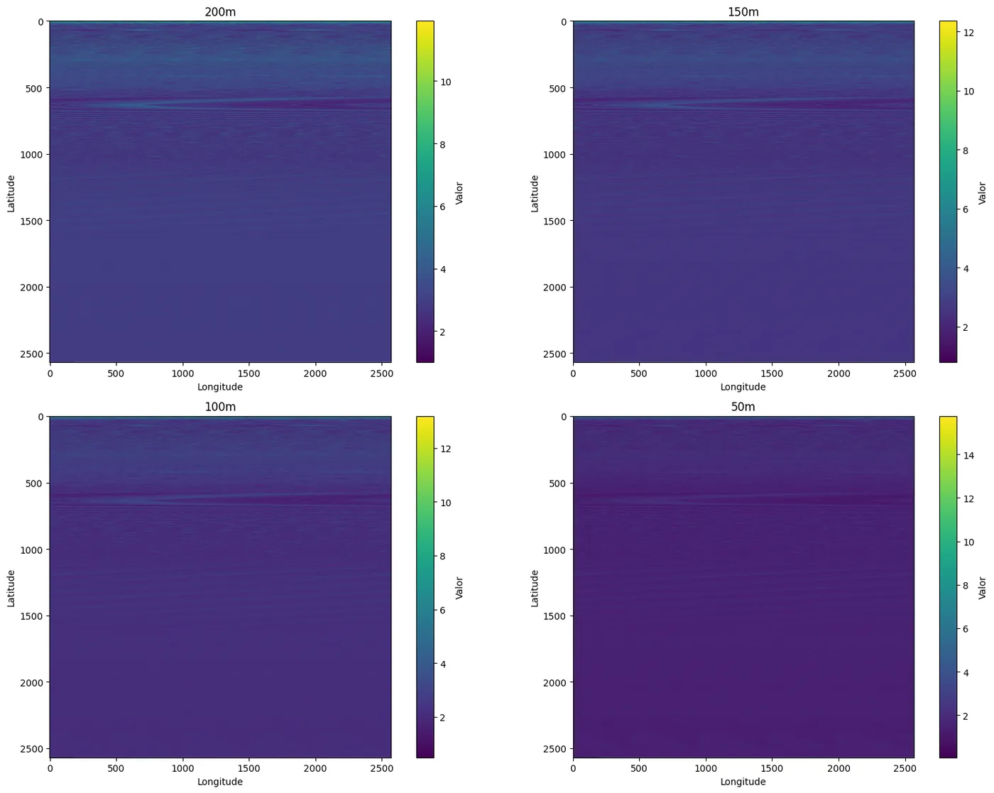
Now we run the structural compression. We generate packed and meta, check the shape of the dense container and save the artifacts. Then we run the round-trip validation, decompressing packed and verifying that the original shape was rebuilt correctly.

compress, meta = compress_raster(stack, nodata)
print("Comprimido:", compress.shape)
print("Meta:", meta)

Comprimido: (5, 2570, 2570) Meta: {'H': 3600, 'W': 5400, 'C': 5, 'idx': array([ 3925721, 3925724, 3925725, ..., 19439997, 19439998, 19439999]), 'N': 6602519, 'h': 2570, 'w': 2570, 'nodata': nan}

band_names = ['200m', '150m', '100m', '50m', '10m']
write_raster('resultado.tif', compress, wind_prof)
save_meta_json(meta, "resultado.meta.json")
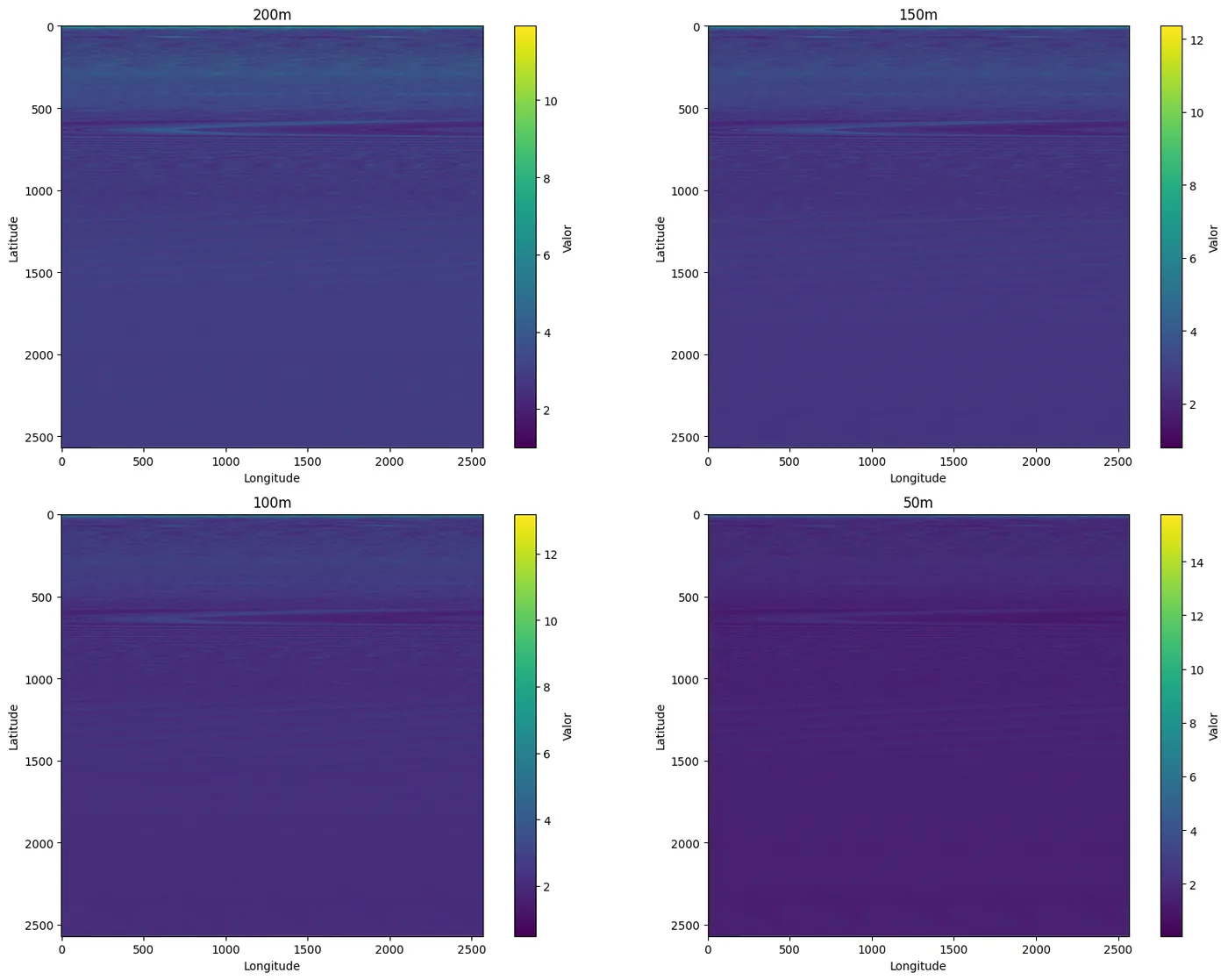
plot_stack(compress, titles=band_names)

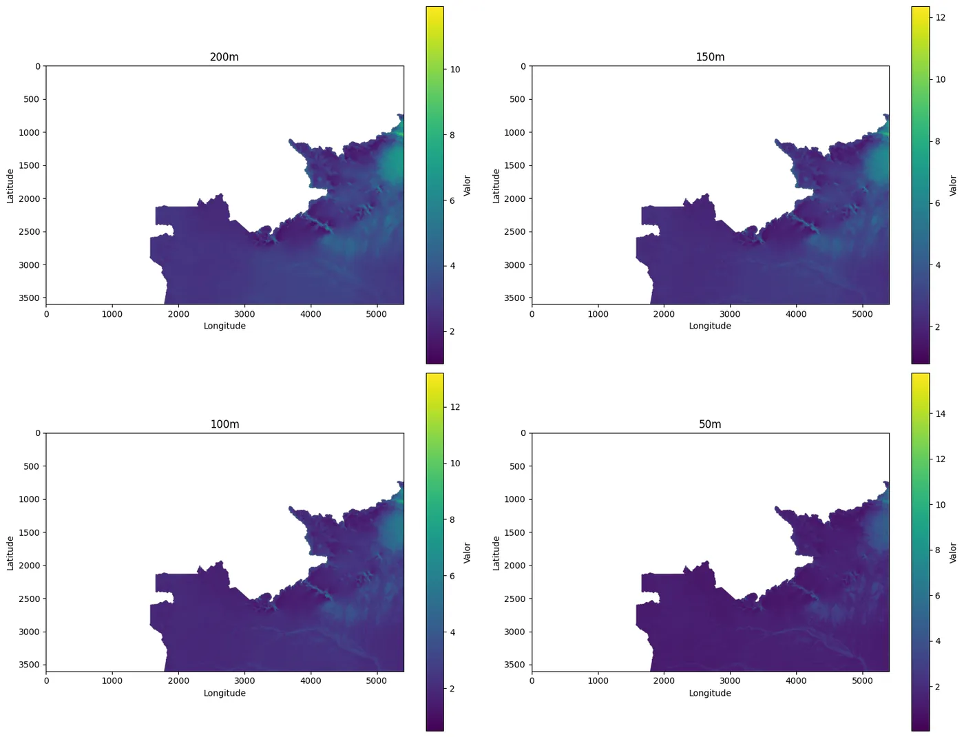
restored= decompress_raster(compress, meta, nodata)
print("Restaurado:", restored.shape)
print(meta)
band_names = ['200m', '150m', '100m', '50m', '10m']
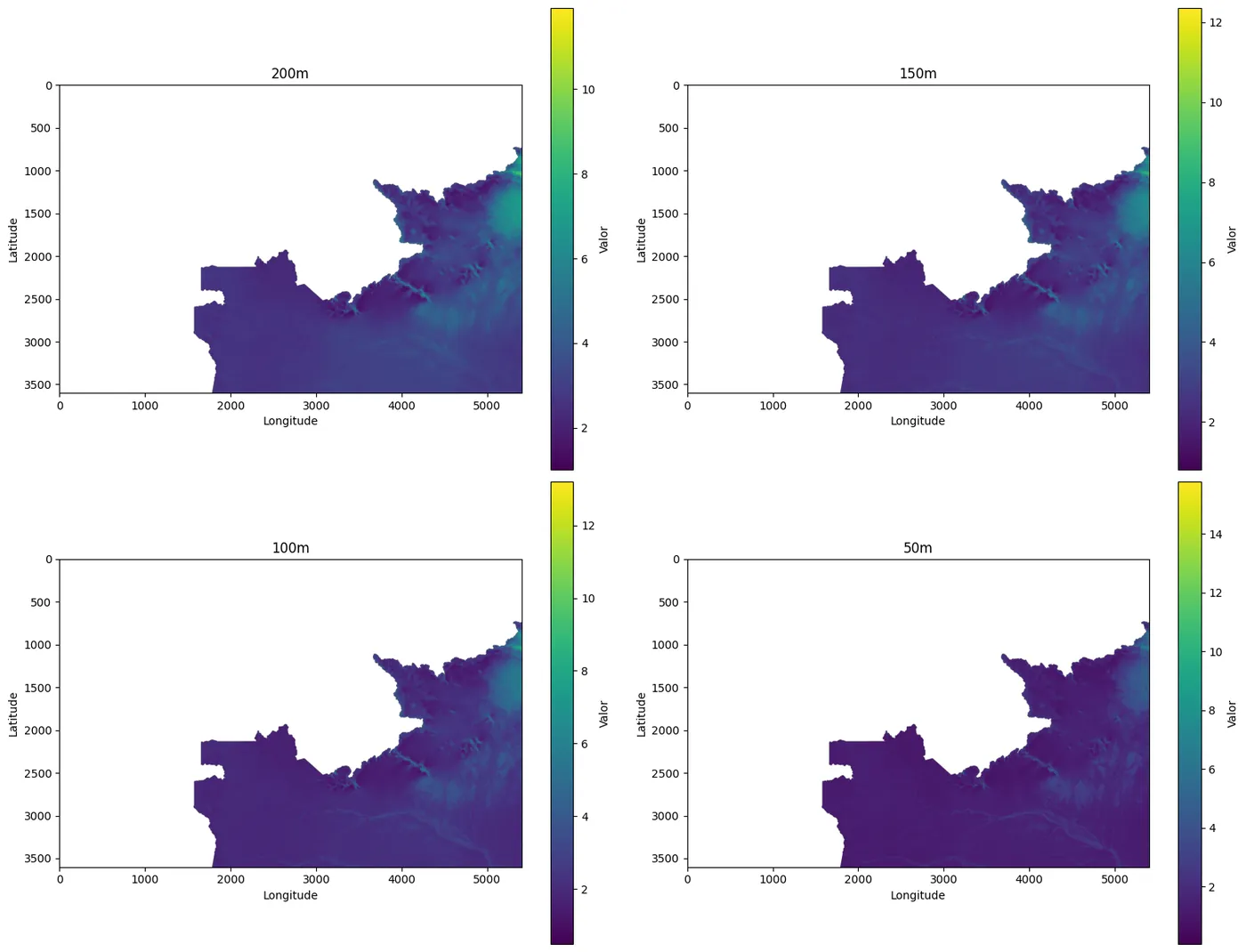
plot_stack(restored, titles=band_names)

Restaurado: (5, 3600, 5400)
{'H': 3600, 'W': 5400, 'C': 5, 'idx': array([ 3925721,  3925724,  3925725, ..., 19439997, 19439998, 19439999]), 'N': 6602519, 'h': 2570, 'w': 2570, 'nodata': nan}

Operating on the compressed data and then decompressing

From here on, we follow a production-ready pattern: we load the compressed array together with its metadata, rehydrate the indices (idx) and operate directly on the dense domain. This reduces scanning cost and speeds up simple operations such as thresholds, filters and mask combinations, especially when the original grid contains large empty areas.

Hey João, can I put this into production?

Yes. That is exactly the idea: you save the compressed image and the metadata artifact (with the reconstruction contract). Later, when you need to go back to the original format, you just use that meta to decompress and rebuild the raster on the same grid, preserving shape, alignment and NoData.

compressed_path = r'/content/resultado.tif'
with rasterio.open(compressed_path) as ds:
        compressed = ds.read()
        profile = ds.profile.copy()

meta_path = r'/content/resultado.meta.json'
meta = load_meta_json(meta_path)
meta['idx'] = np.array(meta['idx'])

plot_stack(compressed, titles=band_names)

decompressed = decompress_raster(compressed, meta, meta['nodata'])
plot_stack(decompressed, titles=band_names)

João, can I operate directly on the compressed raster and only decompress at the end?

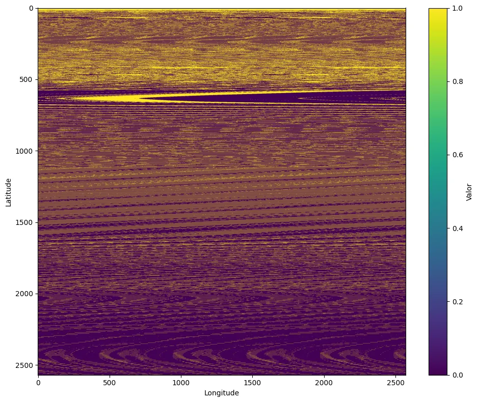
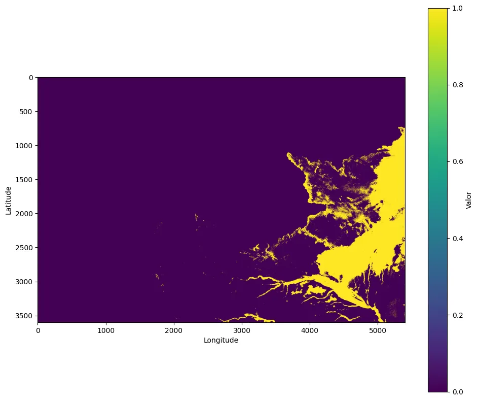
Yes, and that is precisely where the workflow pays off. Let's test it with a simple, common operation: a binary threshold on the 100 m band. First we select the band, define the threshold and create a validity mask in the compressed domain. Then we apply the threshold and produce a 0/1 mask. Finally, we decompress only the binary result to return to the original grid, since that final product is what will be published.

band_idx = 2  # 0=200m,1=150m,2=100m,3=50m,4=10m
thr = 2.4 

band_compress = compressed[band_idx].astype(np.float32)

valid = np.isfinite(band_compress)
if meta.get("nodata") is not None and not (isinstance(meta["nodata"],
                                                      float) and np.isnan(meta["nodata"])):
    valid &= (band_compress != meta["nodata"])

# threshold binário (0/1)
thr_comp = np.zeros_like(band_compress, dtype=np.uint8)
thr_comp[valid & (band_compress >= thr)] = 1

plot_raster(thr_comp)

With our compressed result, the meta file and the NoData value defined, we just call decompress_raster and run the reverse process.

thr_decomp = decompress_raster(thr_comp, meta, nodata)
print("Threshold descomprimido:", thr_decomp.shape, "unique:", np.unique(thr_decomp))
plot_raster(thr_decomp[0])

João, but what is the real advantage in memory usage? Let's compare.

Now we evaluate the RAM cost to understand where the method "pays for itself". To avoid confusion, we clearly separate the concepts. The original stack represents the full cost, proportional to H×W (across all bands), including large empty areas. The compressed array represents the dense domain, where cost becomes proportional to N (only the valid pixels), and that is where operations become cheaper. The restored array exists only to validate the reconstruction contract, which is why it goes back to the same cost as the original stack, since it rehydrates the full H×W grid.

{arrays = {
"stack": stack,
"compressed": compress,
"packed": restored,
}

labels = list(arrays.keys())
sizes_mb = [arr.nbytes / (1024**2) for arr in arrays.values()]

plt.figure(figsize=(8,4))
plt.bar(labels, sizes_mb)
plt.ylabel("Tamanho em RAM (MB)")
plt.tight_layout()
plt.show()

for name, arr in arrays.items():
print(f"{name}: {arr.nbytes/(1024**2):.2f} MB, shape={arr.shape}, dtype={arr.dtype}")}

stack: 370.79 MB, shape=(5, 3600, 5400), dtype=float32
compressed: 125.98 MB, shape=(5, 2570, 2570), dtype=float32
packed: 370.79 MB, shape=(5, 3600, 5400), dtype=float32

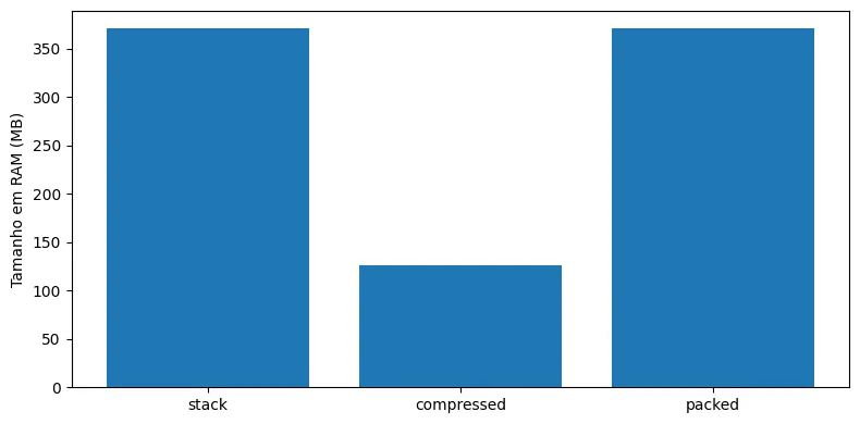
What this comparison shows, quite directly, is the difference between operating on the full domain and operating on the dense domain. Going from 370.79 MB to 125.98 MB, the compressed domain reduces RAM consumption by approximately 66.0%. In other words, the compressed array uses about 34.0% of the memory of the original stack, and it is this reduction that translates into cheaper scans and faster operations day to day.

In production, besides the compressed array, the item that really defines the cost of the contract is idx. It is what allows us to rebuild the original grid, so it needs to be stored and loaded efficiently. When idx is saved as a list in JSON, the file can grow a lot due to serialization overhead. That is why we usually separate small metadata from the large vector.

The most direct way to reduce cost is to store idx in a smaller type when possible. Since the maximum linear index is H×W, if that value fits in uint32, we can cut the cost of idx in half compared to int64. When we also compress the binary file, the gain often grows even further, depending on the structure of the index.

When it makes sense, we can also store the occupancy mask instead of idx. The mask takes H×W bits and can be much smaller on disk. The trade-off is that, at load time, we need to rebuild idx with a flatnonzero operation, which adds a step to loading but keeps the contract working.

Closing the pipeline the production way

In the end, what we built with GetCompress is an intermediate representation that reduces computational cost without losing traceability. We compress once, operate many times on the compressed domain and decompress only when we need to publish a product on the original grid.

The main precaution is not to treat packed as a spatial raster. It is a container. What guarantees integrity is meta, so we treat that metadata as a first-class artifact: we version it alongside the data, validate consistency between N, idx and H×W, and choose a persistence format that does not strangle the gains of the method.

When we follow this pattern, thresholds, masks, filters and statistics no longer scan a gigantic H×W full of emptiness and instead operate on the set of pixels that actually matters. This improves performance and simplifies the production workflow without giving up the original grid.

Reference

ALMAGHRABI, Sarah; RANA, Mashud; HAMILTON, Margaret; RAHAMAN, Mohammad Saiedur. Multivariate solar power time series forecasting using multilevel data fusion and deep neural networks. Information Fusion, v. 104, art. 102180, 2024. DOI: 10.1016/j.inffus.2023.102180