Geospatial GraphRAG Compared to Vector RAG

Translated from the original Portuguese article. Ler o original em português

Projects built on RAG rarely fail for lack of data; the problem is usually something else. The data exists, but the retrieval method does not always support questions that depend on relationships between entities, especially when those relationships are not explicit in the text. In many cases, the system retrieves semantically relevant passages but cannot demonstrate connections such as proximity, territorial co-occurrence, dependency between categories, or a chain of evidence. As a result, the output tends to be a plausible answer that is hard to audit.
In this article, I follow the line of the previous ones and present a pipeline designed to compare, in practice, a traditional vector RAG and a GraphRAG. I will keep using the same OpenStreetMap (OSM) dataset, apply territorial discretization with H3 to it, and build our graph with spatial relationships to support questions that require relational evidence. Instead of only validating the quality of the generated text, we will run an experiment and compare what each approach retrieves, which links it can demonstrate, and how this affects traceability and verification.
The first strategy is a vector baseline. In it, each POI becomes a short document, and retrieval happens through semantic similarity via embeddings. The second strategy is GraphRAG. In this flow, the initial retrieval happens by territorial zones, and the evidence is built by making proximity relationships between categories explicit, with distances and region IDs. In other words, the LLM receives not just items, but pairs and the links between them that justify the answer.
import os, json, time, math, random
from pathlib import Path

import requests
import numpy as np
import pandas as pd
import matplotlib.pyplot as plt

import h3
import re
import networkx as nx
from tqdm import tqdm

import folium
from folium.plugins import MarkerCluster
from pyvis.network import Network

from sklearn.preprocessing import normalize
from sklearn.metrics.pairwise import cosine_similarity

from openai import OpenAI
from google.colab import userdata

os.environ["OPENAI_API_KEY"] = userdata.get("OPENAI_API_KEY")
client = OpenAI()

EMBED_MODEL = "text-embedding-3-small"
LLM_MODEL = "gpt-4o-mini"
Defining the study area and the diagnostic categories
The starting point is to define the spatial extent, with a center in latitude and longitude and a radius in meters, for querying the OSM database. Here we will use a 5 km radius, enough to capture a diverse set of records while still allowing manual inspection of the results on a map.
CENTER_LAT, CENTER_LON = -8.0578, -34.8829
RADIUS_M = 5000
Next, we define the POI categories that provide enough variation and coverage for the test questions. The set includes waste_disposal, recycling, fountain, park and water_point. In general, the goal of this choice is not to represent all of the urban environmental infrastructure, but to form a consistent set of entities for testing relational questions. In addition, to reduce vocabulary fragmentation, drinking_water is normalized to water_point, preventing the same concept from appearing as different categories.
AMENITIES = ["waste_disposal", "recycling", "fountain", "park", "water_point"]

AMENITY_REMAP = {
    "drinking_water": "water_point",
}
Collecting OSM data with Overpass and a local cache
Data collection uses the Overpass API, querying entities through tag filters within the area defined by the search radius.
ROAD_HIGHWAY_REGEX = "^(primary|secondary|tertiary|residential)$"
amenities_regex = "|".join(AMENITIES)

q_pois = f"""
[out:json][timeout:120];
(
  node(around:{RADIUS_M},{CENTER_LAT},{CENTER_LON})["amenity"~"^({amenities_regex})$"];
  way (around:{RADIUS_M},{CENTER_LAT},{CENTER_LON})["amenity"~"^({amenities_regex})$"];
  node(around:{RADIUS_M},{CENTER_LAT},{CENTER_LON})["leisure"="park"];
  way (around:{RADIUS_M},{CENTER_LAT},{CENTER_LON})["leisure"="park"];
  node(around:{RADIUS_M},{CENTER_LAT},{CENTER_LON})["amenity"="drinking_water"];
  way (around:{RADIUS_M},{CENTER_LAT},{CENTER_LON})["amenity"="drinking_water"];
);
out tags center;
"""

q_roads = f"""
[out:json][timeout:120];
way(around:{RADIUS_M},{CENTER_LAT},{CENTER_LON})["highway"~"{ROAD_HIGHWAY_REGEX}"];
out tags geom;
"""

data_pois  = overpass(q_pois,  cache_name=f"pois_env_r{RADIUS_M}_{CENTER_LAT}_{CENTER_LON}", force=True)
data_roads = overpass(q_roads, cache_name=f"roads_r{RADIUS_M}_{CENTER_LAT}_{CENTER_LON}")

print(len(data_pois.get("elements", [])), len(data_roads.get("elements", [])))
To reduce network dependency and make the process easier to rerun, we will create a local cache in JSON format. This avoids repeating calls during iterative adjustments and reduces inconsistencies caused by momentary variations in the API. In addition, the requests are retried with progressive backoff to handle timeouts, rate limits and instability.
def cache_path(name):
    return CACHE_DIR / f"{name}.json"

def overpass(query, cache_name, url=OVERPASS_URL, timeout=180, force=False):
    p = cache_path(cache_name)
    if p.exists() and not force:
        return json.loads(p.read_text(encoding="utf-8"))

    headers = {"User-Agent": "graphrag-ambiental/1.0"}
    last_err = None
    for attempt in range(1, 6):
        try:
            r = requests.post(url, data={"data": query}, headers=headers, timeout=timeout)
            r.raise_for_status()
            data = r.json()
            p.write_text(json.dumps(data), encoding="utf-8")
            return data
        except Exception as e:
            last_err = e
            time.sleep(2 * attempt)
    raise RuntimeError(f"Overpass falhou: {last_err}")
No recorte do exemplo, a coleta retorna 411 POIs e 6.407 vias.
Data preparation and territorial discretization
From the raw data, I extract two DataFrames, one for POIs and another for roads, and then normalize the categories to reduce ambiguity, remove duplicates by osm_id, standardize the coordinates as float, and compute the H3 identifier for each entity, creating a discrete territorial layer.
def extract_pois(elements):
    rows = []
    seen = set()
    for el in elements:
        tags    = el.get("tags", {})
        amenity = tags.get("amenity") or ("park" if tags.get("leisure") == "park" else None)
        if not amenity:
            continue
        amenity = AMENITY_REMAP.get(amenity, amenity)
        if amenity not in AMENITIES:
            continue

        if el["type"] == "node":
            lat, lon = el["lat"], el["lon"]
        else:
            c = el.get("center")
            if not c:
                continue
            lat, lon = c["lat"], c["lon"]

        osm_id = int(el["id"])
        if osm_id in seen:
            continue
        seen.add(osm_id)

        rows.append({
            "osm_type": el["type"],
            "osm_id":   osm_id,
            "amenity":  amenity,
            "name":     tags.get("name"),
            "lat":      float(lat),
            "lon":      float(lon),
        })

    df = pd.DataFrame(rows)
    if df.empty:
        return df
    df["h3"] = df.apply(lambda r: point_to_h3(r["lat"], r["lon"]), axis=1)
    return df

def extract_roads(elements):
    rows = []
    for el in elements:
        if el.get("type") != "way":
            continue
        geom = el.get("geometry")
        if not geom or len(geom) < 2:
            continue
        mid = geom[len(geom)//2]
        tags = el.get("tags", {})
        rows.append({
            "way_id":  int(el["id"]),
            "highway": tags.get("highway"),
            "name":    tags.get("name"),
            "mid_lat": float(mid["lat"]),
            "mid_lon": float(mid["lon"]),
            "geom":    geom,
        })
    df = pd.DataFrame(rows).drop_duplicates(subset=["way_id"])
    df["h3"] = df.apply(lambda r: point_to_h3(r["mid_lat"], r["mid_lon"]), axis=1)
    return df
df_pois = extract_pois(data_pois["elements"])
df_roads = extract_roads(data_roads["elements"])
print(df_pois.shape, df_roads.shape)
Dimensões do DataFrame de POIs (411, 7) e Dimensões do DataFrame de Roads (6407, 7)
We discretize with H3 at resolution 7. This is the step where I stop treating the territory as a continuum and start operating by zones. It makes aggregation, ranking and embedding-based retrieval easier, and it also reduces the search space when I need to build relational evidence.
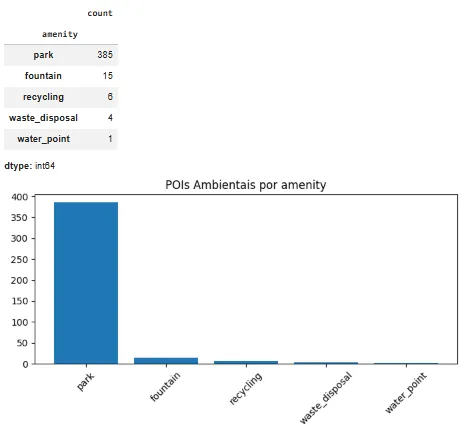
Before moving on, let's take a quick look at the dataset. Counting records per category helps identify imbalances and calibrate expectations.
counts = df_pois["amenity"].value_counts()
display(counts)

plt.figure(figsize=(7, 4))
plt.bar(counts.index, counts.values)
plt.title("POIs Ambientais por amenity")
plt.xticks(rotation=45)
plt.tight_layout()
plt.show()
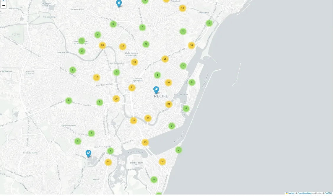
Now let's visualize the data with Folium and MarkerCluster as a sanity check.
m = folium.Map(location=[CENTER_LAT, CENTER_LON], zoom_start=14, tiles="cartodbpositron")
cluster = MarkerCluster().add_to(m)

for r in df_pois.itertuples(index=False):
    folium.Marker(
        location=[r.lat, r.lon],
        popup=f"{r.amenity} | {r.name or 'sem nome'}",
        icon=folium.Icon(icon=ICON_MAP.get(r.amenity, "ok-sign"))
    ).add_to(cluster)

display(m)
Base graph and structural relationships
The graph is, of course, the foundation of GraphRAG, because it materializes relationships that a vector index does not represent explicitly.
G = nx.Graph()
In the adopted model, each POI becomes a node following the pattern poi:, each H3 cell becomes a node zone:
, each category becomes a node svc:, and each road becomes a node road:.
for r in df_pois.itertuples(index=False):
    pid = f"poi:{r.osm_id}"
    G.add_node(pid, ntype="POI", name=r.name, amenity=r.amenity,
               lat=r.lat, lon=r.lon, h3=r.h3)
    G.add_edge(pid, f"zone:{r.h3}",    etype="IN_ZONE")
    G.add_edge(pid, f"svc:{r.amenity}", etype="IS_A")
The graph then receives its structural relationships. The IN_ZONE relationship connects POIs and roads to their H3 zone, while IS_A connects POIs to their service category. Even before adding proximity relationships, this structure already supports questions about zone composition and category distribution.
for r in df_roads.itertuples(index=False):
    rid = f"road:{r.way_id}"
    G.add_node(rid, ntype="ROAD", highway=r.highway, name=r.name,
               lat=r.mid_lat, lon=r.mid_lon, h3=r.h3)
    G.add_edge(rid, f"zone:{r.h3}", etype="IN_ZONE")

print(G.number_of_nodes(), G.number_of_edges())
Tivemos 6839 nodes e 7229 edges
Spatial relationships between POIs by proximity
Most relational questions depend on proximity. That is why we need to create NEAR edges between POIs whenever the distance falls below a threshold, in this case 500 m, capped at 10 neighbors per POI.
MAX_NEAR_M = 500
MAX_NEAR_PER_POI  = 10
To reduce cost, I group the POIs by H3 cell and look for candidates in the cell itself and in one adjacent ring using grid_disk. The distance is computed with Haversine, and the edges store dist_m, which becomes explicit evidence of proximity.
def haversine_m(lat1, lon1, lat2, lon2):
    R = 6371000.0
    p1, p2 = math.radians(lat1), math.radians(lat2)
    dlat = math.radians(lat2 - lat1)
    dlon = math.radians(lon2 - lon1)
    a = math.sin(dlat/2)**2 + math.cos(p1)*math.cos(p2)*math.sin(dlon/2)**2
    return 2 * R * math.atan2(math.sqrt(a), math.sqrt(1 - a))

bucket = {}
for r in df_pois.itertuples(index=False):
    bucket.setdefault(r.h3, []).append(r)

added = 0
for r in tqdm(df_pois.itertuples(index=False), total=len(df_pois)):
    src = f"poi:{r.osm_id}"
    candidates = []
    for c in [r.h3] + list(h3.grid_disk(r.h3, 1)):
        candidates.extend(bucket.get(c, []))
    scored = []
    for t in candidates:
        if t.osm_id == r.osm_id:
            continue
        d = haversine_m(r.lat, r.lon, t.lat, t.lon)
        if d <= MAX_NEAR_M:
            scored.append((d, t.osm_id))
    scored.sort(key=lambda x: x[0])
    for d, tid in scored[:MAX_NEAR_PER_POI]:
        G.add_edge(src, f"poi:{tid}", etype="NEAR", dist_m=float(d))
        added += 1

print(added, G.number_of_edges())
100%|██████████| 411/411 [00:00<00:00, 2540.21it/s]
3529 8359
This part is what sets GraphRAG apart from the vector baseline. The baseline tends to retrieve semantically similar items, but it does not guarantee that they are close to each other in the territory, and by default it does not deliver a set of pairs that satisfies the constraint, which limits what the process can do.
def vector_retrieve(query, k=12):
    q_emb = client.embeddings.create(model=EMBED_MODEL, input=query).data[0].embedding
    q_emb = normalize(np.array(q_emb, dtype=np.float32).reshape(1, -1))
    sims  = cosine_similarity(q_emb, poi_emb)[0]
    idx   = np.argsort(-sims)[:k]
    return [(poi_ids[i], poi_docs[i], float(sims[i])) for i in idx]
Approximate connectivity between roads
Besides proximity between POIs, we also create CONNECTS edges between roads that share sampled points of their geometry. Essentially, the strategy quantizes coordinates to capture approximate intersections and reduce the number of comparisons. Even though this relationship does not directly enter the answer comparison, it adds value by opening the door to future connectivity and accessibility analyses.
ROAD_SAMPLE_STEP = 6

def quantize(lat, lon, ndigits=5):
    return (round(lat, ndigits), round(lon, ndigits))

pt_to_roads = {}
for r in tqdm(df_roads.itertuples(index=False), total=len(df_roads)):
    for p in r.geom[::ROAD_SAMPLE_STEP]:
        key = quantize(p["lat"], p["lon"])
        pt_to_roads.setdefault(key, set()).add(r.way_id)

connects = 0
for key, roads in pt_to_roads.items():
    roads = list(roads)
    if len(roads) < 2:
        continue
    for i in range(min(len(roads), 10)):
        for j in range(i + 1, min(len(roads), 10)):
            G.add_edge(f"road:{roads[i]}", f"road:{roads[j]}", etype="CONNECTS")
            connects += 1

print(connects)
100%|██████████| 6407/6407 [00:00<00:00, 138242.22it/s]
1785
Documents and embeddings for the vector baseline
In the vector baseline, each POI is represented as a short text document containing its ID, name, category, coordinates and H3 zone. Explicitly including the ID, the H3 cell and the coordinates helps reduce ambiguity when the LLM needs to justify a location.
def poi_doc(row):
    name = row["name"] if pd.notnull(row["name"]) else "sem nome"
    return (
        f"Ativo de Infraestrutura Ambiental ID {row['osm_id']}: {name}. "
        f"Categoria={row['amenity']}. "
        f"Localização (lat={row['lat']:.6f}, lon={row['lon']:.6f}). "
        f"Zona territorial H3={row['h3']}."
    )

poi_docs = df_pois.apply(poi_doc, axis=1).tolist()
poi_ids  = df_pois["osm_id"].tolist()
Next, we generate the embeddings of these documents using the text-embedding-3-small model and measure similarity with cosine similarity. When a question arrives, its embedding is computed and compared against the vector corpus. The most similar items are then selected and used as context for the generation step.
EMBED_MODEL = "text-embedding-3-small"
LLM_MODEL = "gpt-4o-mini"

def embed_texts(texts, model=EMBED_MODEL, batch_size=128):
    vecs = []
    for i in tqdm(range(0, len(texts), batch_size)):
        batch = texts[i:i + batch_size]
        resp = client.embeddings.create(model=model, input=batch)
        vecs.extend([d.embedding for d in resp.data])
    return np.array(vecs, dtype=np.float32)

poi_emb = embed_texts(poi_docs)
print(poi_emb.shape)
100%|██████████| 4/4 [00:01<00:00, 2.08it/s](411, 1536)
This flow is simple and efficient. It works well when the question is descriptive or asks for a list. The limitation shows up when the query requires a verifiable relationship, such as proximity between categories. In that case, semantic similarity may retrieve items that are correct in theme but geographically scattered, without forming pairs that satisfy the constraint. The model then ends up inferring connections from text rather than from structural evidence.
def vector_retrieve(query, k=12):
    q_emb = client.embeddings.create(model=EMBED_MODEL, input=query).data[0].embedding
    q_emb = normalize(np.array(q_emb, dtype=np.float32).reshape(1, -1))
    sims  = cosine_similarity(q_emb, poi_emb)[0]
    idx   = np.argsort(-sims)[:k]
    return [(poi_ids[i], poi_docs[i], float(sims[i])) for i in idx]

def baseline_answer(query, k=12):
    top = vector_retrieve(query, k=k)
    ctx = "\n".join([f"- {pid} | score={s:.3f} | {doc}" for pid, doc, s in top])
    prompt = (
        "Você é um assistente GeoAI especializado em diagnóstico de infraestrutura ambiental urbana para apoio a decisões públicas e estratégias ESG. Responda SOMENTE com os POIs fornecidos.\n"
        "Se pedir 'perto', use h3/lat/lon como aproximação e explique.\n"
        "Responda em bullets estruturados.\n"
        "Cite sempre os IDs dos ativos ambientais.\n"
        "Inclua interpretação territorial quando possível.\n"
        f"PERGUNTA:\n{query}\n\nCONTEXTO:\n{ctx}"
    )
    return llm_text(prompt), top
Zones as documents in GraphRAG and summaries
In GraphRAG, on the other hand, retrieval does not start with individual entities but with territorial zones. Each H3 cell is turned into a document that summarizes the profile of the area, including the total number of assets and the predominant categories. For the densest zones, the LLM generates a short executive summary focused on characterizing the territorial pattern in a clear and structured way.
This summary step has two main goals. First, to improve the quality of embedding-based retrieval, since texts describing a zone's profile tend to represent its context better than plain counts. Second, to make explicit that this is a reading based on open data, so the summary is not mistaken for an official or exhaustive diagnosis.
zone_stats = (
    df_pois.groupby(["h3", "amenity"])
    .size()
    .reset_index(name="n")
    .sort_values(["h3", "n"], ascending=[True, False])
)
zone_total = df_pois.groupby("h3").size().reset_index(name="total")

zone_card = {}
for h, grp in zone_stats.groupby("h3"):
    top_svc = ", ".join([f"{r.amenity}:{int(r.n)}" for r in grp.head(8).itertuples(index=False)])
    total   = int(zone_total.loc[zone_total["h3"] == h, "total"].iloc[0])
    zone_card[h] = (
        f"Zona territorial H3={h} (resolução={H3_RES}). "
        f"Total de ativos ambientais mapeados={total}. "
        f"Principais categorias de infraestrutura ambiental={top_svc}."
    )

dense_zones = zone_total.sort_values("total", ascending=False)["h3"].head(60).tolist()

def summarize_zone(h):
    prompt = (
        f"Gere um sumário executivo curto (2-4 frases) para apoio a decisão pública "
        f"sobre a infraestrutura ambiental desta zona territorial.\n"
        f"Baseie-se APENAS nos dados:\n{zone_card[h]}\n"
        f"Inclua:\n"
        f"(1) Perfil da infraestrutura ambiental local,\n"
        f"(2) Possível vocação territorial (ex.: lazer, gestão de resíduos, suporte hídrico),\n"
        f"(3) Indique que se trata de uma estimativa baseada em dados abertos."
    )
    return llm_text(prompt)

zone_summary = {}
for h in tqdm(dense_zones):
    zone_summary[h] = summarize_zone(h)

def zone_text(h):
    return zone_summary.get(h, zone_card.get(h, f"Zona H3={h}"))
zone_list = list(zone_card.keys())
zone_docs = [zone_text(h) for h in zone_list]
zone_emb  = normalize(embed_texts(zone_docs))
print(len(zone_list), zone_emb.shape)
100%|██████████| 1/1 [00:00<00:00,  2.88it/s]
15 (15, 1536)
Understanding the question and controlled extraction
In relational questions, a common failure is not the LLM failing to answer. The failure is the process not translating the question into retrievable constraints. To reduce this risk, we will use a JSON schema to extract the services, the pairs of services that must be close to each other, the radius in meters, a place hint, and the number of zones for the initial retrieval.
QUERY_SCHEMA = {
    "type": "object",
    "additionalProperties": False,
    "properties": {
        "services": {
            "type": "array",
            "items": {"type": "string", "enum": AMENITIES},
        },
        "near_pairs": {
            "type": "array",
            "items": {
                "type": "object",
                "additionalProperties": False,
                "properties": {
                    "a":        {"type": "string", "enum": AMENITIES},
                    "b":        {"type": "string", "enum": AMENITIES},
                    "radius_m": {"type": "integer", "minimum": 50, "maximum": 5000},
                },
                "required": ["a", "b", "radius_m"],
            },
        },
        "place_hint":  {"type": "string"},
        "top_k_zones": {"type": "integer", "minimum": 1, "maximum": 25},
    },
    "required": ["services", "near_pairs", "place_hint", "top_k_zones"],
}
We also need a parsing function that enforces limits and default values, avoiding unrealistic radii and making sure vague questions do not break the flow. It also applies a fallback: when the question mentions at least two services but no proximity pair comes back, I create a default pair with a radius, preserving the relational nature of the problem.
def parse_query(query):
    prompt = (
        "Extraia estrutura da pergunta no JSON abaixo.\n"
        "Não invente serviços fora do enum.\n\n"
        "REGRAS OBRIGATÓRIAS:\n"
        "- radius_m deve ser entre 50 e 5000. Se não especificado, use 500.\n"
        "- top_k_zones deve ser entre 1 e 25. Se não especificado, use 8.\n"
        "- Se a pergunta mencionar PROXIMIDADE, INTEGRAÇÃO, SINERGIA ou 'perto' "
        "entre dois tipos de serviço, SEMPRE preencha near_pairs com o par correspondente.\n"
        "  Exemplos de mapeamento:\n"
        "    'áreas verdes' ou 'parques' ou 'lazer'-'park'\n"
        "    'reciclagem'                           -'recycling'\n"
        "    'ativos hídricos' ou 'água' ou 'fonte'-'water_point' ou 'fountain'\n"
        "    'descarte' ou 'lixo' ou 'resíduos'    -'waste_disposal'\n"
        "- Se houver dois serviços identificados em contexto de proximidade, "
        "gere um near_pair com esses dois serviços.\n\n"
        f"Schema: {json.dumps(QUERY_SCHEMA)}\n"
        f"Pergunta: {query}\n"
        "Responda SOMENTE com JSON válido, sem markdown."
    )
    raw = llm_text(prompt)
    raw = raw.replace("```json", "").replace("```", "").strip()
    q = json.loads(raw)

    q["top_k_zones"] = max(1, min(25, int(q.get("top_k_zones") or 8)))
    for p in q.get("near_pairs", []):
        p["radius_m"] = max(50, min(5000, int(p.get("radius_m") or 500)))

    # Fallback: se services tem ≥2 itens e near_pairs ainda vazio
    svcs = q.get("services", [])
    if not q.get("near_pairs") and len(svcs) >= 2:
        q["near_pairs"] = [{"a": svcs[0], "b": svcs[1], "radius_m": 500}]

    return q
How does GraphRAG build evidence?
GraphRAG operates in two layers. In the first, it retrieves the most relevant zones using zone embeddings. Instead of searching individual POIs directly, it ranks the H3 cells whose profile best matches the question, reducing the search space and avoiding a sweep of the entire territory.
def retrieve_zones(query, topk=10):
    q_emb = client.embeddings.create(model=EMBED_MODEL, input=query).data[0].embedding
    q_emb = normalize(np.array(q_emb, dtype=np.float32).reshape(1, -1))
    sims  = cosine_similarity(q_emb, zone_emb)[0]
    idx   = np.argsort(-sims)[:topk]
    return [(zone_list[i], zone_docs[i], float(sims[i])) for i in idx]
In the second layer, I build relational evidence within that subset. It filters the POIs contained in the retrieved zones and applies service category constraints. When the question involves proximity between categories, it gradually expands the H3 search ring until it reaches sufficient coverage or hits a limit. With the candidate set defined, I compute nearby pairs between the requested categories within the given radius and record the distance in meters, which becomes explicit evidence to support the answer.
def build_evidence(services, near_pairs, zones_ranked, max_evidence=40, max_ring=2):
    slices = [df_pois[df_pois["h3"].isin(list(h3.grid_disk(h, ZONE_RING)))]
              for h, _, _ in zones_ranked]
    slices = [s for s in slices if not s.empty]
    if not slices:
        return pd.DataFrame(), []
    cand = pd.concat(slices, ignore_index=True).drop_duplicates(subset=["osm_id"])

    if services:
        cand = cand[cand["amenity"].isin(services)]

    evid = []
    if near_pairs:
        # Tenta rings crescentes até achar POIs de ambos os tipos
        ring_df = pd.DataFrame()
        for ring in range(0, max_ring + 1):
            ring_slices = [df_pois[df_pois["h3"].isin(list(h3.grid_disk(h, ring)))]
                           for h, _, _ in zones_ranked]
            ring_slices = [s for s in ring_slices if not s.empty]
            if not ring_slices:
                continue
            candidate = pd.concat(ring_slices, ignore_index=True).drop_duplicates(subset=["osm_id"])

            needed = {p["a"] for p in near_pairs} | {p["b"] for p in near_pairs}
            found  = set(candidate["amenity"].unique())
            if needed.issubset(found):
                ring_df = candidate
                break  # ring suficiente encontrado

        if ring_df.empty:
            # Usa tudo disponível no dataset nas zonas
            ring_df = pd.concat([
                df_pois[df_pois["h3"].isin(list(h3.grid_disk(h, max_ring)))]
                for h, _, _ in zones_ranked
            ], ignore_index=True).drop_duplicates(subset=["osm_id"])

        by_am    = {a: ring_df[ring_df["amenity"] == a].copy() for a in AMENITIES}
        keep_ids = set()

        for p in near_pairs:
            A = by_am.get(p["a"]); B = by_am.get(p["b"])
            if A is None or B is None or len(A) == 0 or len(B) == 0:
                print(f"  near_pair {p['a']}↔{p['b']}: "
                      f"{len(A) if A is not None else 0} tipo-A, "
                      f"{len(B) if B is not None else 0} tipo-B (sem pares possíveis)")
                continue
            B_pts = list(B[["osm_id", "lat", "lon"]].itertuples(index=False))
            for ra in A[["osm_id", "lat", "lon", "name"]].itertuples(index=False):
                dists = [(haversine_m(ra.lat, ra.lon, rb.lat, rb.lon), rb.osm_id)
                         for rb in B_pts
                         if haversine_m(ra.lat, ra.lon, rb.lat, rb.lon) <= p["radius_m"]]
                dists.sort()
                if dists:
                    keep_ids.add(int(ra.osm_id))
                    for d, bid in dists[:5]:
                        keep_ids.add(int(bid))
                        evid.append((int(ra.osm_id), int(bid), float(d),
                                     f"NEAR({p['a']},{p['b']})"))

        cand = ring_df[ring_df["osm_id"].isin(list(keep_ids))].copy()

    return cand.head(max_evidence), evid
Finally, I assemble the context sent to the LLM in three blocks. The first summarizes the retrieved zones and their scores. The second lists the filtered POIs with ID, category, coordinates and H3 cell. The third describes the relationships found, including the pairs and their distances. In practice, this shifts the model's job from inventing connections to explaining connections that have already been verified, whereas the vector baseline tends to retrieve semantically similar items and leaves the construction of the link to the generation step.
def graphrag_answer(query):
    q            = parse_query(query)
    zones_ranked = retrieve_zones(query, topk=int(q["top_k_zones"]))
    df_ev, edges = build_evidence(q["services"], q["near_pairs"], zones_ranked)

    zone_ctx = "\n".join([f"- Zona {h} | score={s:.3f} | {zone_card[h]}"
                          for h, _, s in zones_ranked[:8]])
    poi_ctx  = "\n".join([
        f"- POI {r.osm_id}: {r.amenity} | {r.name or 'sem nome'} | "
        f"lat={r.lat:.6f}, lon={r.lon:.6f} | h3={r.h3}"
        for r in df_ev.itertuples(index=False)
    ]) if not df_ev.empty else "Nenhum POI encontrado nas zonas recuperadas."
    edge_ctx = "\n".join([f"- POI {a} -> POI {b} | {rel} | dist_m={d:.1f}"
                          for a, b, d, rel in edges[:80]])

    prompt = (
        "Você é um assistente GeoAI especializado em diagnóstico de infraestrutura ambiental urbana. "
        "Responda SOMENTE com base no contexto abaixo.\n"
        "As respostas devem apoiar decisão pública ou análise ESG.\n"
        "Não faça inferências além dos dados listados.\n"
        "Se não houver evidência suficiente, indique claramente a limitação.\n\n"
        f"PERGUNTA:\n{query}\n\n"
        f"ZONAS:\n{zone_ctx}\n\n"
        f"POIs:\n{poi_ctx}\n\n"
        f"RELAÇÕES:\n{edge_ctx}"
    )
    return llm_text(prompt), q, zones_ranked, df_ev, edges
Visualizing the results on the map
So that we can actually see the results when comparing the two approaches, we will add a visualization step. The idea is simple: plot the retrieved POIs and, when there is relational evidence, draw the links between nearby pairs. This makes manual inspection easier and helps quickly spot limitations in the retrieval process.
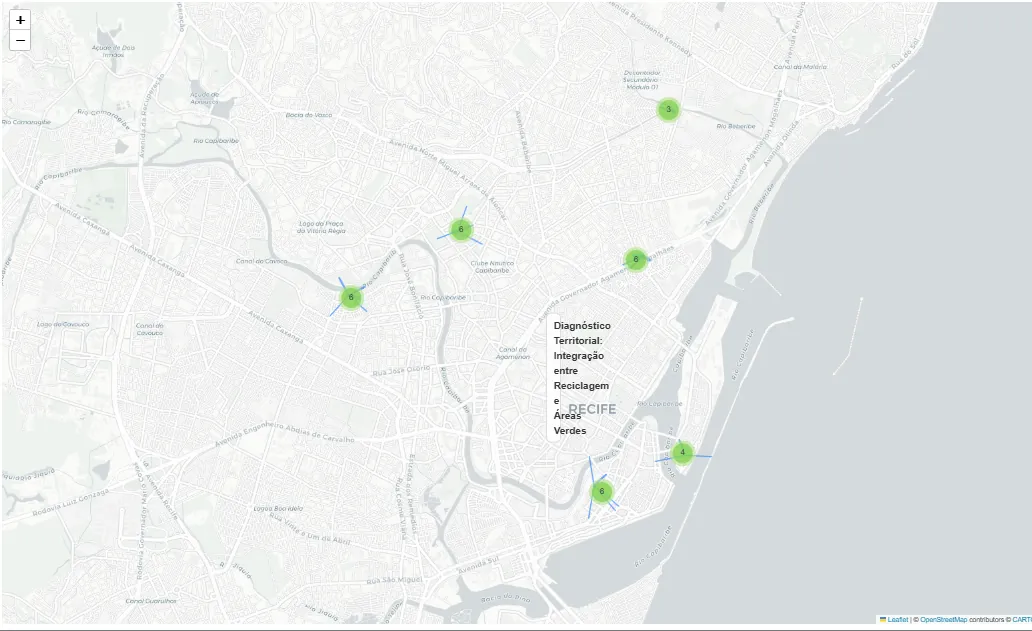
In the vector baseline, the visualization shows only the POIs returned by the similarity search. Since there are no explicit relationships in this flow, the map mainly serves to check territorial dispersion.
def show_baseline_on_map(top_base, title="Baseline Recuperado"):
    ids = [pid for pid, _, _ in top_base]
    df_base = df_pois[df_pois["osm_id"].isin(ids)].copy()

    m = folium.Map(location=[CENTER_LAT, CENTER_LON], zoom_start=14, tiles="cartodbpositron")

    for r in df_base.itertuples(index=False):
        folium.Marker(
            location=[r.lat, r.lon],
            popup=f"{r.amenity} | {r.name or 'sem nome'} | POI {r.osm_id}",
            icon=folium.Icon(icon=ICON_MAP.get(r.amenity, "ok-sign"))
        ).add_to(m)

    return m
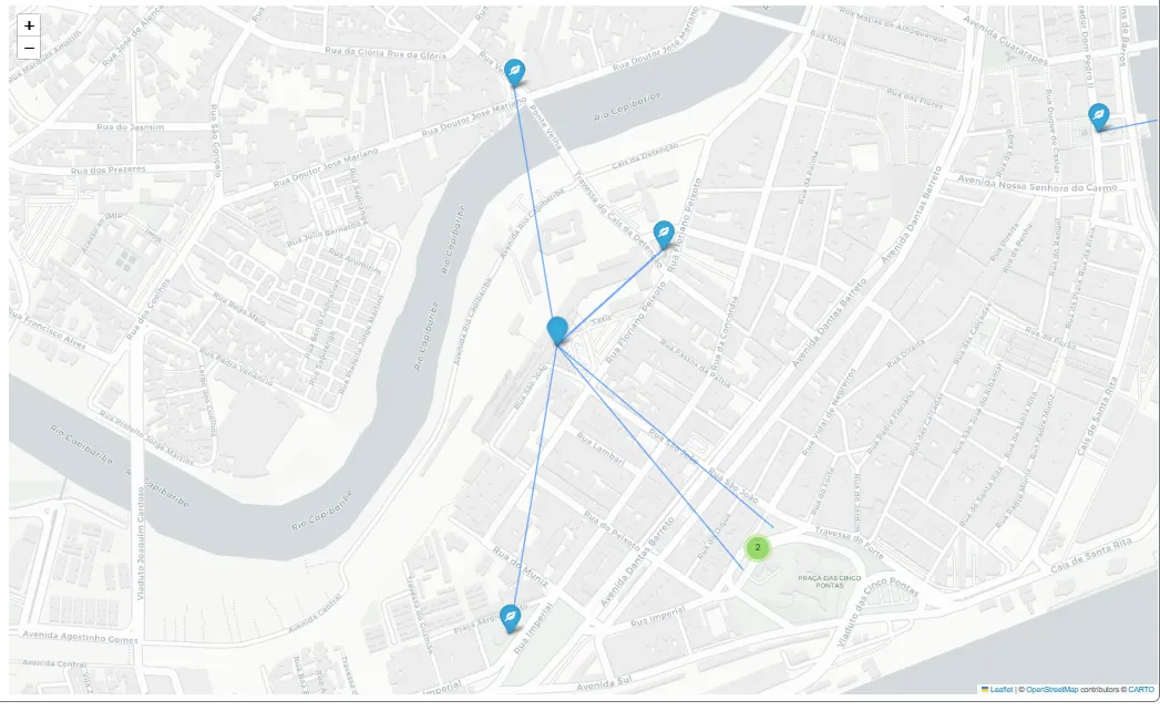
For GraphRAG, the visualization also includes the edges: lines are drawn between the POIs that satisfy the proximity constraint, illustrating the distances between them.
def show_subgraph(df_ev, edges, title="Subgrafo GraphRAG Ambiental",
                  center=None, zoom=16, max_nodes=80, max_edges=200):
    if df_ev.empty or "osm_id" not in df_ev.columns:
        print(f"[show_subgraph] Nenhuma evidência para exibir: '{title}'")
        return None

    nodes = df_ev.head(max_nodes).copy()
    nodes["osm_id"] = nodes["osm_id"].astype(int)
    idx = {int(r.osm_id): (float(r.lat), float(r.lon), str(r.amenity), r.name or "sem nome")
           for r in nodes.itertuples(index=False)}

    if center is None:
        lats = [v[0] for v in idx.values()]
        lons = [v[1] for v in idx.values()]
        center = (sum(lats) / len(lats), sum(lons) / len(lons))

    m = folium.Map(location=list(center), zoom_start=zoom, tiles="cartodbpositron")
    folium.map.Marker(
        list(center),
        icon=folium.DivIcon(html=(
            f'{title}'
        ))
    ).add_to(m)

    cl = MarkerCluster().add_to(m)
    for oid, (lat, lon, amenity, name) in idx.items():
        folium.Marker(
            location=[lat, lon],
            popup=f"{amenity} | {name} | POI {oid}",
            icon=folium.Icon(icon=ICON_MAP.get(amenity, "ok-sign"))
        ).add_to(cl)

    drawn = 0
    for a, b, d, rel in edges:
        if drawn >= max_edges:
            break
        a, b = int(a), int(b)
        if a not in idx or b not in idx:
            continue
        lat1, lon1, *_ = idx[a]
        lat2, lon2, *_ = idx[b]
        w = 5 if float(d) <= 150 else 3 if float(d) <= 300 else 2
        folium.PolyLine(
            locations=[[lat1, lon1], [lat2, lon2]],
            weight=w, opacity=0.65,
            tooltip=f"{rel}: {a}→{b} | {float(d):.1f}m"
        ).add_to(m)
        drawn += 1

    m.fit_bounds([[min(v[0] for v in idx.values()), min(v[1] for v in idx.values())],
                  [max(v[0] for v in idx.values()), max(v[1] for v in idx.values())]])
    return m
Comparative experiment and evaluation
For the experiment, we will use explicitly relational questions. They explicitly involve proximity between categories, demanding more than simple thematic retrieval. The goal is to observe how each approach responds when the question depends on a verifiable link between entities.
For each question, we run both the vector baseline and GraphRAG, recording not only the answer texts but also the IDs, the ranked zones, the pairs found, and the subset of evidence used in generation. This way, the comparison is not limited to narrative quality. It considers what each method actually retrieves and with what structural support.
The questions used in the test focus on surveying and analyzing environmental infrastructure:
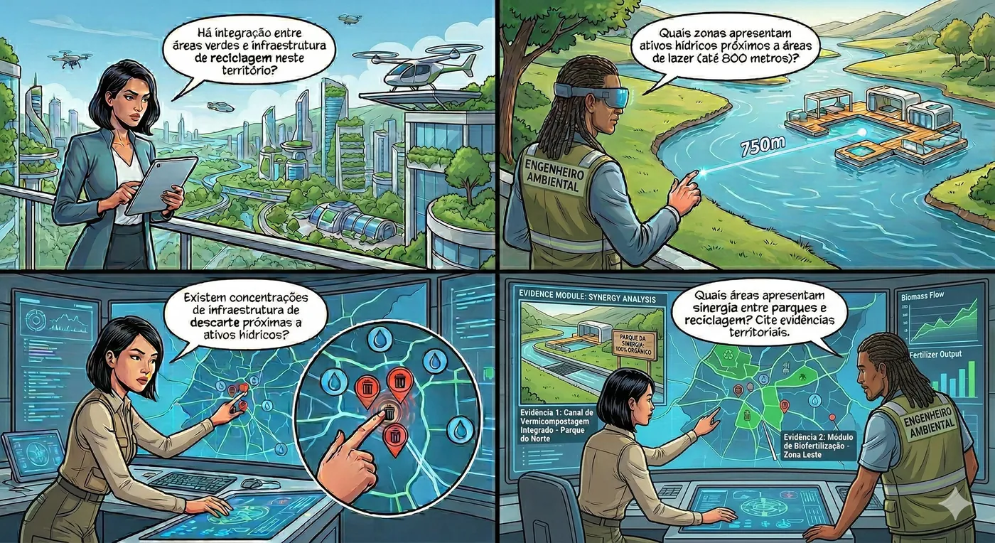
TEST_QUERIES = [
    "Há integração entre áreas verdes e infraestrutura de reciclagem neste território?",
    "Quais zonas apresentam ativos hídricos próximos a áreas de lazer (até 800 metros)?",
    "Existem concentrações de infraestrutura de descarte próximas a ativos hídricos?",
    "Quais áreas apresentam sinergia entre parques e reciclagem? Cite evidências territoriais.",
]
With the test questions defined, the next step is to run both approaches for each question and consolidate the results into a comparable structure that includes the text answers and the retrieved evidence:
rows = []
for q in TEST_QUERIES:
    base_ans, base_top                    = baseline_answer(q, k=14)
    graph_ans, qobj, zones, df_ev, edges  = graphrag_answer(q)
    rows.append({
        "query":            q,
        "baseline_answer":  base_ans,
        "graphrag_answer":  graph_ans,
        "baseline_top_ids": [x[0] for x in base_top[:8]],
        "graphrag_ev_ids":  df_ev["osm_id"].head(12).tolist() if "osm_id" in df_ev.columns else [],
        "zones_top":        [z[0] for z in zones[:5]],
        "edges":            edges,
        "df_ev":            df_ev,
    })

df_compare = pd.DataFrame(rows)
df_compare.head()
| query | baseline_answer | graphrag_answer | baseline_top_ids | graphrag_ev_ids | zones_top | edges | df_ev |
|---|---|---|---|---|---|---|---|
| Há integração entre áreas verdes e infraestrutura de reciclagem neste território? | Sim, há integração entre áreas verdes e infraestrutura de reciclagem neste território. Várias zonas possuem parques próximos a pontos de reciclagem, com distâncias que variam de 34.4 metros a 498.5 metros. | Sim, há integração entre áreas verdes e infraestrutura de reciclagem neste território. | [12920110239, 5792360470, 678531198, 660899644, 607806652, 12519405586, 660889443, 667128528] | [12519405586, 242165865, 673508120, 12920110239, 666315850, 666315851, 666323889, 666323891, 666323892, 666323893, 666323894, 666504517] | [878183995ffffff, 878183998ffffff, 878183983ffffff, 87818399cffffff, 878183986ffffff] | (666315850, 678531198, 341.1171043269651, NEAR(park,recycling)) | osm_type | osm_id | amenity ... |
| Quais zonas apresentam ativos hídricos próximos a áreas de lazer (até 800 metros)? | As zonas que apresentam ativos hídricos próximos a áreas de lazer (até 800 metros) são: Zona 878183981ffffff com distâncias de 259.5m a 712.2m. | As zonas que apresentam ativos hídricos próximos a áreas de lazer são: 878183981ffffff. | [8319557555, 544598870, 660902380, 678541451, 655717658, 854786879, 673243750, 660886154] | [673223374, 673223375, 673504760, 8319557555, 199886985, 446100758] | [87818399effffff, 878183984ffffff, 8781839b1ffffff, 878183980ffffff, 87818398effffff] | (8319557555, 446100758, 259.51782203347364, NEAR(water_point,park)) | osm_type | osm_id | amenity ... |
| Existem concentrações de infraestrutura de descarte próximas a ativos hídricos? | Com base nas informações fornecidas, existem concentrações de infraestrutura de descarte (waste_disposal) nas zonas 878183983ffffff, 87818399cffffff e 878183998ffffff. | Existem concentrações de waste_disposal próximas a ativos hídricos. | [1023718706, 1024258938, 1023700587, 1023664089, 8319557555, 5792360470, 12920110239, 678531198] | [] | [878183986ffffff, 878183983ffffff, 878183981ffffff, 878183980ffffff, 878183982ffffff] | [] | Empty DataFrame |
| Quais áreas apresentam sinergia entre parques e reciclagem? Cite evidências territoriais. | As áreas que apresentam sinergia entre parques e reciclagem são: Zona 878183995ffffff (10 parques, 1 reciclagem); Zona 87818399cffffff (30 parques, 1 reciclagem); Zona 878183983ffffff (30 parques, 1 reciclagem). | As áreas com sinergia incluem 878183995ffffff, 87818399cffffff e 878183983ffffff. | [580584425, 377386145, 666323894, 128476663, 128476662, 662611662, 128476682, 1318429777] | [12519405586, 242165865, 673508120, 582306392, 1037707118, 1037707119, 12920110239, 666315850, 666315851, 666323889, 666323891, 666323892] | [878183998ffffff, 878183995ffffff, 87818399cffffff, 878183983ffffff, 878183984ffffff] | (367630671, 5792360470, 418.04369139438927, NEAR(park,recycling)) | osm_type | osm_id | amenity ... |
In the tests run with these questions, the difference between the approaches becomes clear. In some cases, the vector baseline returns items that are semantically consistent with the theme of the query but does not present explicit pairs that prove the requested relationship. The connection between the elements appears in the text, but it is not necessarily backed by structural evidence.
GraphRAG, on the other hand, tends to produce answers that are more firmly anchored in verifiable links. Even when the text is more concise, it comes with pairs that have a measurable distance and with the identification of the zones involved. This makes the answer more auditable, since it lets us trace exactly which entities were connected and under which spatial criterion.
I also run a few targeted unit tests to inspect the behavior of each approach in isolation. For example, when asking which recycling points are near parks, I can look at the baseline result as text and, in the case of GraphRAG, inspect the generated subgraph on the map:
ans_base, top_base = baseline_answer(
    "Quais pontos de reciclagem ficam perto de parques?"
)

display(show_baseline_on_map(top_base, title="Baseline - Reciclagem e Parques"))
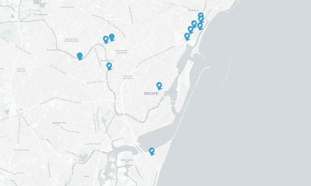
ans_g, qobj, zones, df_ev, edges = graphrag_answer(
    "Quais pontos de reciclagem ficam perto de parques?"
)
display(show_subgraph(df_ev, edges, title="Diagnóstico Territorial: Integração entre Reciclagem e Áreas Verdes"))
To ensure a repeatable and structured evaluation, we set up an LLM to act as a judge, using an explicit validation schema. This judge measures criteria such as groundedness (how well the answer is grounded in the provided context) and adherence to constraints, for example, answering exclusively based on the provided context and correctly citing the relevant IDs.
Although this approach does not replace human review, it makes it possible to identify patterns, inconsistencies and early deviations in a systematic and scalable way.
JUDGE_SCHEMA = {
    "type": "object",
    "additionalProperties": False,
    "properties": {
        "groundedness":        {"type": "integer", "minimum": 1, "maximum": 5},
        "constraint_following":{"type": "integer", "minimum": 1, "maximum": 5},
        "notes":               {"type": "string"},
    },
    "required": ["groundedness", "constraint_following", "notes"],
}

def judge(query, answer, evidence_ids):
    prompt = (
        "Avalie a resposta de um assistente geoespacial e retorne JSON válido "
        f"com este schema: {json.dumps(JUDGE_SCHEMA)}\n\n"
        f"Pergunta: {query}\n\n"
        f"Resposta:\n{answer}\n\n"
        f"Evidências (IDs de POIs recuperados):\n{evidence_ids}\n\n"
        "Critérios:\n"
        "- groundedness: 1..5 (resposta parece baseada nas evidências)\n"
        "- constraint_following: 1..5 (cita IDs, respeita 'somente contexto')\n"
        "- notes: 1-3 frases\n"
        "Responda SOMENTE com JSON, sem markdown."
    )
    raw = llm_text(prompt)
    raw = raw.replace("```json", "").replace("```", "").strip()
    return json.loads(raw)
Let's call the judge to measure and check how well the answers adhere to the criteria.
scores = []
for r in rows:
    s_base  = judge(r["query"], r["baseline_answer"], r["baseline_top_ids"])
    s_graph = judge(r["query"], r["graphrag_answer"],  r["graphrag_ev_ids"])
    scores.append({
        "query":                    r["query"],
        "baseline_groundedness":    s_base["groundedness"],
        "baseline_constraints":     s_base["constraint_following"],
        "baseline_notes":           s_base["notes"],
        "graphrag_groundedness":    s_graph["groundedness"],
        "graphrag_constraints":     s_graph["constraint_following"],
        "graphrag_notes":           s_graph["notes"],
    })

df_scores = pd.DataFrame(scores)
display(df_scores[[
    "query",
    "baseline_groundedness", "baseline_constraints",
    "graphrag_groundedness",  "graphrag_constraints",
]])

# médias por método
print("\nMédias:")
print(f"  Baseline: groundedness: {df_scores['baseline_groundedness'].mean():.2f} | constraints: {df_scores['baseline_constraints'].mean():.2f}")
print(f"  GraphRAG: groundedness: {df_scores['graphrag_groundedness'].mean():.2f} | constraints: {df_scores['graphrag_constraints'].mean():.2f}")
| query | baseline_groundedness | baseline_constraints | graphrag_groundedness | graphrag_constraints |
|---|---|---|---|---|
| 0 | 4 | 5 | 5 | 5 |
| 1 | 3 | 4 | 5 | 5 |
| 2 | 4 | 5 | 4 | 4 |
| 3 | 5 | 5 | 5 | 5 |
The LLM judge evaluation shows that GraphRAG matched or exceeded the baseline averages: a groundedness of 4.75 versus 4.00, and constraint adherence of 4.75 for both methods. The baseline varied more across queries (in query 1, for example, it scored 3 on groundedness), while GraphRAG kept high scores in most of them, which indicates good textual coherence, proper citation of IDs, and compliance with the prompt instructions.
However, this metric evaluates the alignment between the answer and the provided context, not the structural quality of the retrieved relationships. GraphRAG may score lower when it returns more conservative answers or explicitly points out coverage limitations, as in query 2. On top of that, it provides verifiable links and measurable distances, something the textual judge does not fully capture. That is why the analysis needs to be complemented with relational metrics, which evaluate whether the requested relationships were actually retrieved.
Relational metric with precision and recall
Since the goal of GraphRAG is to retrieve relationships, the evaluation needs to check whether the returned pairs actually correspond to valid relationships in the graph. To do this, we define two core functions for the comparison, ground_truth_pairs and relational_accuracy.
The ground_truth_pairs function builds the reference set for each combination of categories and radius defined in the query. It iterates over the NEAR edges already in the graph and keeps only those that connect two POIs of the requested categories and respect the maximum distance. The result is a set of unique ID pairs representing all valid relationships in the territory for that constraint. This set works as an operational ground truth, independent of the embedding-based retrieval process.
def ground_truth_pairs(near_pairs_def, radius_m=500):

    gt = set()
    for u, v, data in G.edges(data=True):
        if data.get("etype") != "NEAR":
            continue
        d = data.get("dist_m", 9999)
        if d > radius_m:
            continue
        # extrai tipo de cada nó
        u_data = G.nodes[u]; v_data = G.nodes[v]
        if u_data.get("ntype") != "POI" or v_data.get("ntype") != "POI":
            continue
        for p in near_pairs_def:
            conds = [
                (u_data.get("amenity") == p["a"] and v_data.get("amenity") == p["b"]),
                (u_data.get("amenity") == p["b"] and v_data.get("amenity") == p["a"]),
            ]
            if any(conds) and d <= p["radius_m"]:
                uid = int(u.split(":")[1]); vid = int(v.split(":")[1])
                gt.add((min(uid, vid), max(uid, vid)))
    return gt
Next, the relational_accuracy function compares the pairs actually retrieved by GraphRAG against this reference set. From that comparison, it computes precision, recall and F1. Precision measures how many of the retrieved pairs are actually valid. Recall measures how many of the existing valid pairs were found. F1 balances the two, offering a single summary view of relational performance.
def relational_accuracy(retrieved_edges, gt_pairs):
    """
    Precision  = pares recuperados que estão no GT / total recuperados
    Recall     = pares recuperados que estão no GT / total no GT
    F1         = média harmônica
    """
    if not retrieved_edges or not gt_pairs:
        return {"precision": 0.0, "recall": 0.0, "f1": 0.0,
                "tp": 0, "retrieved": len(retrieved_edges), "gt_size": len(gt_pairs)}

    retrieved_norm = {(min(int(a), int(b)), max(int(a), int(b)))
                      for a, b, *_ in retrieved_edges}
    tp = len(retrieved_norm & gt_pairs)
    precision = tp / len(retrieved_norm) if retrieved_norm else 0.0
    recall    = tp / len(gt_pairs)       if gt_pairs    else 0.0
    f1 = (2 * precision * recall / (precision + recall)
          if (precision + recall) > 0 else 0.0)
    return {
        "precision": round(precision, 4),
        "recall":    round(recall,    4),
        "f1":        round(f1,        4),
        "tp":        tp,
        "retrieved": len(retrieved_norm),
        "gt_size":   len(gt_pairs),
    }
Now let's apply it to the tests and compute the metrics.
NEAR_PAIRS_DEFAULT = [{"a": a, "b": b, "radius_m": RADIUS_M}
                      for a in AMENITIES for b in AMENITIES if a < b]

ras_rows = []
for q in TEST_QUERIES:
    ans_g, qobj, zones, df_ev, edges = graphrag_answer(q)

    near_pairs = qobj.get("near_pairs") or NEAR_PAIRS_DEFAULT
    gt   = ground_truth_pairs(near_pairs, radius_m=max((p["radius_m"] for p in near_pairs), default=MAX_NEAR_M))
    ras  = relational_accuracy(edges, gt)

    ras_rows.append({"query": q[:60] + "...", **ras})

df_ras = pd.DataFrame(ras_rows)
print("\nRELATIONAL ACCURACY SCORE ")
display(df_ras[["query", "precision", "recall", "f1", "tp", "retrieved", "gt_size"]])

print("\nMédias")
print(df_ras[["precision", "recall", "f1"]].mean().round(4).to_string())
| query | precision | recall | f1 | tp | retrieved | gt_size |
|---|---|---|---|---|---|---|
| 0 | 0.7714 | 0.8438 | 0.8060 | 27 | 35 | 32 |
| 1 | 0.4000 | 1.0000 | 0.5714 | 2 | 5 | 2 |
| 2 | 0.0000 | 0.0000 | 0.0000 | 0 | 0 | 0 |
| 3 | 0.7714 | 0.8438 | 0.8060 | 27 | 35 | 32 |
The results show different behaviors across the queries. In queries 0 and 3, there is a good balance between precision and recall, with an F1 score of 0.8060 in both. This indicates that the system managed to retrieve mostly correct relationships while keeping satisfactory coverage of the reference set, with 27 out of 32 valid relationships identified in each. In these cases, there is consistency between what exists in the graph and what was actually retrieved.
In query 1, the picture is different. Recall is 1.0, meaning that all relevant relationships were found. However, precision is 0.4, showing that a significant share of the returned pairs does not belong to the valid set. The system was comprehensive, but it introduced noise by including relationships that do not strictly satisfy the defined constraint.
Query 2 has an F1 of 0, but with a gt_size of 0, which indicates that there are no expected relationships in the territory for that combination of categories and radius. In this case, the result is semantically neutral, since there were no relationships to retrieve. The zero value comes from the mathematical definition of the metrics, not from a retrieval error.
As for the averages, a precision of 0.4857, a recall of 0.6719 and an F1 of 0.5459 show that the system tends to retrieve a good share of the relevant relationships, with recall higher than precision. This suggests a strategy that is more sensitive than specific. Coverage is good, but there is still considerable noise, which leaves room for improvement.
Final thoughts
The baseline, that is, vector RAG, is efficient, simple and computationally cheaper. It works well for descriptive or listing questions, where semantic similarity is enough to retrieve the relevant entities. Its main limitation appears when the query requires verifiable links, such as proximity or integration, because it may return items that are individually correct, leaving the LLM to infer connections that are not explicitly supported.
GraphRAG, on the other hand, adds a structural layer to the retrieval process. By operating on zones and building pairs with measurable distances, it turns the constraints in the question into evidence, increasing traceability. In the end, the test made it clear to me that the two methods do not compete directly; rather, each one is better suited to a different kind of problem. When the question is relational and requires proof of a link, the graph-based approach tends to be more appropriate. When the task is predominantly descriptive and cost needs to be kept low, vector RAG is definitely the better choice.