Beyond Latitude and Longitude: Creating Spatial Embeddings for RAG

Translated from the original Portuguese article. Ler o original em português

When I started combining large language models (LLMs) with geographic data, my first temptation was to treat latitude and longitude as "just two more features" and move on. I soon saw the problem: coordinates are great, but they do not capture context. Latitude and longitude say nothing about neighborhood. They do not capture the notion of proximity well, they do not work as discrete identities, and they do not offer a clear hierarchical structure, such as district, street and block, which makes that connection hard to establish.
In this article, I share a simple, practical way to turn location into something that behaves like an embedding, that is, a vector representation that can be indexed, compared and used for retrieval. Best of all, the process is fully deterministic, requires no training, is cheap and scales well. To do this, we will use H3, the spatial indexing library created by Uber, which is widely used for operations and analysis on vector layers.
Defining the study area: Recife as an example
To make the explanation more concrete, I chose to work with an area of Recife and points of interest from OpenStreetMap (OSM). From this dataset, I built a basic geographic retrieval and then took the next step of combining geography and text to create a consistent geographic RAG base, something an LLM can use effectively.
Before fetching the data, I needed to define the scope of the experiment. In geoprocessing, this matters more than it seems, because the study area influences density, the types of places and even the behavior of the retrieval. In my case, I defined an approximate bounding box for Recife.
# Recife
SOUTH, WEST, NORTH, EAST = -8.15, -35.02, -7.95, -34.85
With the area defined, I queried OSM points through the Overpass API. I selected categories that are common in urban environments, such as hospital, school, pharmacy, police and shelter. These classes are easy to validate and represent the dynamics of the city well. This gave me a dataset that is both realistic and interpretable.
import requests, pandas as pd

OVERPASS_URL = "https://overpass-api.de/api/interpreter"
AMENITIES = ["hospital", "school", "pharmacy", "police", "shelter"]

query = f"""
[out:json][timeout:60];
(
  node["amenity"~"^({'|'.join(AMENITIES)})$"]({SOUTH},{WEST},{NORTH},{EAST});
);
out center;
"""

resp = requests.post(OVERPASS_URL, data=query)
data = resp.json()
len(data["elements"])
1250
Structuring the data for indexing
With the data collected, I organized everything into a format that is easy to index and debug, building a DataFrame with the essential columns, such as id, name, category, latitude and longitude. It may seem trivial, but this step makes life much easier later on, especially when you want to evolve the pipeline, for example by switching from node to way or relation and using center instead of the direct coordinates.
rows = []
for el in data["elements"]:
    tags = el.get("tags", {})
    amenity = tags.get("amenity")
    name = tags.get("name", None)

    if el["type"] == "node":
        lat, lon = el.get("lat"), el.get("lon")
    else:
        center = el.get("center", {})
        lat, lon = center.get("lat"), center.get("lon")

    rows.append({
        "osm_type": el["type"],
        "osm_id": el["id"],
        "name": name,
        "category": amenity,
        "lat": lat,
        "lon": lon
    })

df = pd.DataFrame(rows)
df.head()
| Index | OSM Type | OSM ID | Name | Category | Latitude | Longitude |
|---|---|---|---|---|---|---|
| 0 | node | 560397916 | - | pharmacy | -8.0624473 | -34.8964475 |
| 1 | node | 560398646 | Colégio GGE | school | -8.0620287 | -34.8987418 |
| 2 | node | 560400267 | Delegacia de Polícia Civil | police | -8.0458839 | -34.9275611 |
| 3 | node | 560628925 | Colégio Sancarlos | school | -8.0477011 | -34.9282542 |
| 4 | node | 561522263 | Colégio Souza Leão | school | -8.0541609 | -34.9198574 |
When analyzing the class distribution, I noticed that schools dominate the dataset. That is actually a good thing, because it creates a situation close to reality. When searching for a class like hospital, I do not want to get nearby schools just because they are the majority. In other words, the retrieval needs to understand intent, not just density.
df["category"].value_counts()
| Category | Count |
|---|---|
| school | 720 |
| hospital | 193 |
| pharmacy | 158 |
| shelter | 105 |
| police | 74 |
Up to this point, I only had a set of points with latitude and longitude. This is where the central shift comes in: instead of treating coordinates as continuous numbers, we convert them into spatial tokens with H3.
Converting coordinates into spatial tokens with H3
!pip install h3
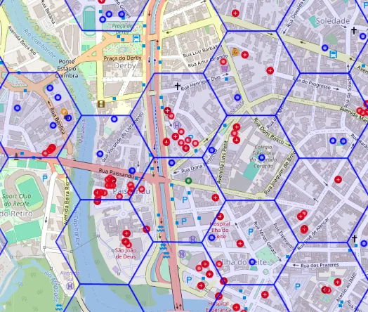
The core idea of H3 is to divide the map into hexagons and assign a unique identifier to each cell, as in the image alongside. For the LLM, this identifier works as a spatial token.
When using this index, you can choose different resolutions, representing space at multiple scales. I used resolutions 7, 9 and 11 to capture everything from broader regions down to local detail.
import h3

def add_h3(df: pd.DataFrame, res: int) -> pd.DataFrame:
    out = df.copy()
    out[f"h3_r{res}"] = [
        h3.latlng_to_cell(lat, lon, res) for lat, lon in zip(out["lat"], out["lon"])
    ]
    return out

df = add_h3(df, 7)
df = add_h3(df, 9)
df = add_h3(df, 11)
df[["lat","lon","h3_r7","h3_r9","h3_r11"]].head()
| Index | Latitude | Longitude | H3 R7 | H3 R9 | H3 R11 |
|---|---|---|---|---|---|
| 0 | -8.0624473 | -34.8964475 | 878183980ffffff | 89818398053ffff | 8b818398051cfff |
| 1 | -8.0620287 | -34.8987418 | 878183980ffffff | 89818398057ffff | 8b8183980573fff |
| 2 | -8.0458839 | -34.9275611 | 878183981ffffff | 8981839810fffff | 8b81839810ebfff |
| 3 | -8.0477011 | -34.9282542 | 878183981ffffff | 89818398107ffff | 8b8183981050fff |
| 4 | -8.0541609 | -34.9198574 | 878183981ffffff | 898183981cfffff | 8b8183981cf5fff |
From here on, each location is no longer just a point and is instead represented by a set of discrete identifiers. This is when the embedding starts to take shape, without the need to train a network.
Dealing with the edge problem
In the real world, edges matter. Two points can be very close but fall into different hexagons. If those hexagons are treated as completely distinct, retrieval tends to fail exactly where it should succeed.
To deal with this, I adopted a simple strategy: in addition to the token of the main cell, I also included the tokens of the neighboring cells. In H3, this set is called a k-ring, or grid disk. I used resolution 9 as the urban base and k = 1 to include the immediate neighbors.
First, I generated a multiscale signature. Then I expanded that signature with the neighboring cells. This way, the concept of "near" is no longer limited to distance and starts to incorporate topological adjacency, which improves performance in dense areas.
RESOLUTIONS = (7, 9, 11)

def spatial_signature(lat: float, lon: float, resolutions=RESOLUTIONS):
    return [h3.latlng_to_cell(lat, lon, r) for r in resolutions]

df["sig"] = [spatial_signature(lat, lon) for lat, lon in zip(df["lat"], df["lon"])]

df["sig"].head()
sig
0 [878183980ffffff, 89818398053ffff, 8b818398051...
1 [878183980ffffff, 89818398057ffff, 8b818398057...
2 [878183981ffffff, 8981839810fffff, 8b81839810e...
3 [878183981ffffff, 89818398107ffff, 8b818398105...
4 [878183981ffffff, 898183981cfffff, 8b8183981cf...
And then expand it with neighbors:
def sig_with_neighbors(sig, k=1):
    base = sig[1]  # r9
    nbrs = list(h3.grid_disk(base, k))
    return sig + nbrs

df["sig_k1"] = [sig_with_neighbors(s, k=1) for s in df["sig"]]
df["sig_k1"].head()
sig_k1
0 878183980ffffff
89818398053ffff
8b818398...
1 878183980ffffff
89818398057ffff
8b818398...
2 878183981ffffff
8981839810fffff
8b818398...
3 878183981ffffff
89818398107ffff
8b818398...
4 878183981ffffff
898183981cfffff
8b818398...
Turning everything into vectors (hashing trick)
With the tokens defined, the next step was to convert them into fixed-dimension numeric vectors. This makes it possible to use cosine similarity and vector indexes such as FAISS or HNSW and, consequently, to apply RAG.
For this conversion, I used the hashing trick, where each token is mapped to a position in the vector through a hash function, MD5 in this case, accumulating counts at that position. At the end, I normalize the vector. The result was a set of 1,250 locations in Recife converted into vectors ready for retrieval.
import numpy as np, hashlib

def hash_to_idx(token: str, dim: int) -> int:
    h = hashlib.md5(token.encode("utf-8")).hexdigest()
    return int(h, 16) % dim

def tokens_to_vec(tokens, dim=1024):
    v = np.zeros(dim, dtype=np.float32)
    for t in tokens:
        v[hash_to_idx(t, dim)] += 1.0
    n = np.linalg.norm(v)
    return v if n == 0 else (v / n)

DIM = 1024
V_geo = np.vstack([tokens_to_vec(toks, dim=DIM) for toks in df["sig_k1"].values])
V_geo.shape
(1250, 1024)
Visualizing the retrieval on the map
After turning the points into vectors and structuring the index, I wanted to observe the spatial behavior of the system. To do so, I defined a query point and visualized on the map which locations the retrieval mechanism considered closest.
I used a Python function with matplotlib:
def plot_retrieval(query_lat, query_lon, results, title="", margin=0.01):
    plt.figure(figsize=(10, 8))
    ax = plt.gca()

    # Calcular bounds da região de interesse
    all_lats = np.concatenate([results["lat"].values, [query_lat]])
    all_lons = np.concatenate([results["lon"].values, [query_lon]])

    lat_min, lat_max = all_lats.min() - margin, all_lats.max() + margin
    lon_min, lon_max = all_lons.min() - margin, all_lons.max() + margin

    # Filtrar pontos de contexto que estão na região visível
    context_mask = (
        (df["lat"] >= lat_min) & (df["lat"] <= lat_max) &
        (df["lon"] >= lon_min) & (df["lon"] <= lon_max)
    )
    context_df = df[context_mask]

    # Pontos de contexto (cinza claro, pequenos)
    ax.scatter(
        context_df["lon"].values,
        context_df["lat"].values,
        s=20,
        c='lightgray',
        alpha=0.5,
        label='Outros pontos na região',
        zorder=1
    )

    # Top-k retornado (azul, médios)
    ax.scatter(
        results["lon"].values,
        results["lat"].values,
        s=100,
        c='royalblue',
        edgecolors='darkblue',
        linewidths=1.5,
        label='Resultados (top-k)',
        zorder=3
    )

    # Ponto da query (vermelho, grande)
    ax.scatter(
        [query_lon],
        [query_lat],
        s=250,
        c='red',
        marker='*',
        edgecolors='darkred',
        linewidths=2,
        label='Query',
        zorder=4
    )

    # Linhas da query para cada resultado
    for _, r in results.iterrows():
        ax.plot(
            [query_lon, r["lon"]],
            [query_lat, r["lat"]],
            'b-',
            alpha=0.3,
            linewidth=1,
            zorder=2
        )

    # Definir limites do plot
    ax.set_xlim(lon_min, lon_max)
    ax.set_ylim(lat_min, lat_max)

    # Adicionar anotações para os top 3
    for i, row in results.head(3).iterrows():
        ax.annotate(
            f"{i+1}. {row['name'][:20] if pd.notna(row['name']) else row['category']}\n(score: {row['score']:.3f})",
            xy=(row['lon'], row['lat']),
            xytext=(10, 10),
            textcoords='offset points',
            fontsize=8,
            bbox=dict(boxstyle='round,pad=0.5', fc='yellow', alpha=0.7),
            arrowprops=dict(arrowstyle='->', connectionstyle='arc3,rad=0', lw=1)
        )

    ax.set_title(title, fontsize=12, fontweight='bold')
    ax.set_xlabel("Longitude", fontsize=10)
    ax.set_ylabel("Latitude", fontsize=10)
    ax.legend(loc='upper right', fontsize=9)
    ax.grid(True, alpha=0.3)

    # Aspect ratio igual para lat/lon
    ax.set_aspect('equal', adjustable='box')

    plt.tight_layout()
    plt.show()
"Near me" retrieval with vector similarity
Retrieval is the process of fetching relevant information from an indexed dataset. In vector systems, this means identifying the items most similar to a query based on a metric, such as cosine similarity or Euclidean distance.
First, we create the geographic retriever to start testing proximity-based retrieval, by computing the similarity against the whole dataset.
This approach does not aim to measure distances in meters with absolute precision (which would be slow with many points); the goal is to provide a practical notion of proximity that is fast, indexable and less sensitive to edge effects. In many urban contexts, this level of approximation is enough, especially for use cases like "Which hospital is closest to this coordinate?".
from sklearn.metrics.pairwise import cosine_similarity

def retrieve_geo(query_lat, query_lon, topk=10):
    q_tokens = sig_with_neighbors(spatial_signature(query_lat, query_lon), k=1)
    q_vec = tokens_to_vec(q_tokens, dim=DIM).reshape(1, -1)

    sims = cosine_similarity(q_vec, V_geo).ravel()
    top = np.argsort(-sims)[:topk]

    out = df.iloc[top][["name", "category", "lat", "lon"]].copy()
    out["score"] = sims[top]
    return out.reset_index(drop=True)

query_lat = float(df.iloc[0].lat)
query_lon = float(df.iloc[0].lon)

res_geo = retrieve_geo(query_lat, query_lon, topk=10)
display(res_geo)

plot_retrieval(
    query_lat, query_lon, res_geo,
    title=f"Retrieval GEO | lat={query_lat:.6f}, lon={query_lon:.6f} | topk=10"
)
| Index | Name | Category | Latitude | Longitude | Score |
|---|---|---|---|---|---|
| 0 | - | pharmacy | -8.0624473 | -34.8964475 | 1.000000238418579 |
| 594 | Real Hospital Português | hospital | -8.0643955 | -34.8981574 | 0.9166668653488159 |
| 605 | Instituto Cervantes | school | -8.0617243 | -34.8971303 | 0.9166668653488159 |
| 603 | - | hospital | -8.0631268 | -34.8953544 | 0.9166668653488159 |
| 589 | - | hospital | -8.0627699 | -34.8983415 | 0.9166668653488159 |
| 584 | - | hospital | -8.0628958 | -34.898804 | 0.6172134876251221 |
| 1231 | Hospital Memorial São José | hospital | -8.0598305 | -34.8971396 | 0.5833334922790527 |
| 1 | colégio GGE | school | -8.0620287 | -34.8987418 | 0.5833334922790527 |
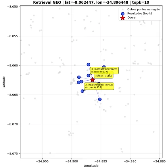
Obviously, this is not perfect: notice that it still selected some classes that are not hospitals. Also, if a user searched right on the border between two neighborhoods, there could be some confusion. But in practice, this is a process that can work well enough for most everyday cases.
Combining text and geography: the step that creates geographic RAG
Up to this point, I was answering the question "what is near this coordinate?". However, the user's real question is usually different: "which hospitals are near me?".
To incorporate semantic intent into the search, I generated text embeddings from the name and category using the SentenceTransformer model. I chose the all-MiniLM-L6-v2 model, which for me offered a good balance between performance and computational cost; it is very lightweight and ran well on my machine. Then I concatenated the textual and geographic embeddings.
from sentence_transformers import SentenceTransformer

model = SentenceTransformer("all-MiniLM-L6-v2")

texts = (df["name"].fillna("") + " " + df["category"].fillna("")).tolist()
V_txt = model.encode(texts, normalize_embeddings=True)

V_hybrid = np.hstack([V_txt, V_geo])
V_hybrid.shape
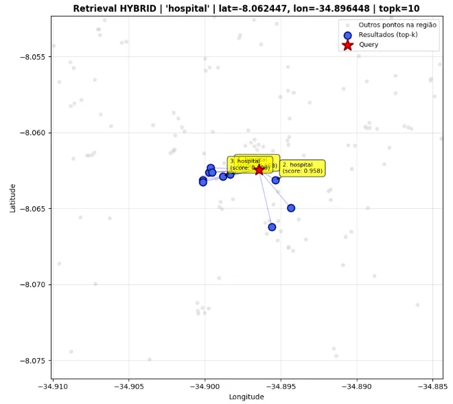
When I analyzed the result, the gain was immediate. The system is no longer purely geographic and starts to consider location and intent at the same time. Instead of returning any nearby point, it prioritizes what is both nearby and semantically aligned with the query.
Now we truly have a geographic RAG. The retriever selects the most appropriate context, and the LLM takes over the linguistic step, explaining, comparing or recommending based on the retrieved results.
def retrieve_hybrid(query_text, query_lat, query_lon, topk=10):
    # texto
    q_txt = model.encode([query_text], normalize_embeddings=True)

    # geo
    q_tokens = sig_with_neighbors(spatial_signature(query_lat, query_lon), k=1)
    q_geo = tokens_to_vec(q_tokens, dim=DIM).reshape(1, -1)

    # concat
    q = np.hstack([q_txt, q_geo])

    sims = cosine_similarity(q, V_hybrid).ravel()
    top = np.argsort(-sims)[:topk]

    out = df.iloc[top][["name", "category", "lat", "lon"]].copy()
    out["score"] = sims[top]
    return out.reset_index(drop=True)

query_text = "hospital"

res_hybrid = retrieve_hybrid(query_text, query_lat, query_lon, topk=10)
display(res_hybrid)

plot_retrieval(
    query_lat, query_lon, res_hybrid,
    title=f"Retrieval HYBRID | '{query_text}' | lat={query_lat:.6f}, lon={query_lon:.6f} | topk=10"
)
| Index | Name | Category | Latitude | Longitude | Score |
|---|---|---|---|---|---|
| 589 | - | hospital | -8.0627699 | -34.8983415 | 0.9583333730697632 |
| 603 | - | hospital | -8.0631268 | -34.8953544 | 0.9583333730697632 |
| 584 | - | hospital | -8.0628958 | -34.898804 | 0.808606743812561 |
| 604 | - | hospital | -8.0649677 | -34.8943472 | 0.7916668057441711 |
| 597 | - | hospital | -8.0631409 | -34.9001382 | 0.7916668057441711 |
| 587 | - | hospital | -8.0626232 | -34.8997285 | 0.7916668057441711 |
| 636 | - | hospital | -8.0662101 | -34.895579 | 0.7916668057441711 |
| 672 | - | hospital | -8.0623306 | -34.8996346 | 0.7916668057441711 |
Conclusion
Here I started from a clear limitation of coordinates. When used on their own, latitude and longitude do not adequately represent context. By converting space into multiscale H3 tokens, incorporating adjacency with the k-ring and turning these signatures into vectors through the hashing trick, I built a simple, deterministic and efficient geographic embedding. This process requires no training, has low computational cost and scales predictably.
The most relevant point, however, is not just technical. By turning location into a vector representation compatible with modern retrieval mechanisms, we start treating space as part of the system's language. Geography stops being an external filter and becomes part of the model's own reasoning.
When this embedding is combined with textual representations generated by SentenceTransformer, the result is a retriever capable of understanding both what is being searched for and where. At this stage, geographic RAG is no longer an ad hoc adaptation and operates as an integrated architecture, bringing together location and semantic intent in a practical way that applies to real-world contexts, from urban contextual search to intelligent decision-support systems.
In the end, this goes beyond spatial indexing: it is a way to make LLMs truly understand geography rather than just describe coordinates, an essential step for LLMs to stop merely describing space and actually begin to understand it.