

Updated 2026 (published in 2021)
Genetic algorithm, random search, TPE and CMA-ES: which method finds better hyperparameters

Translated from the original Portuguese article. Ler o original em português

We already learn that a model's default settings are rarely the best, and that it is worth spending some time tuning the hyperparameters. But I wondered how much that tuning really pays off, and whether a smarter search method beats simply drawing configurations at random. I also wanted to see a genetic algorithm I wrote myself in the same fight as the methods that Optuna ships ready to use.
I set up the experiment with the same budget for everyone, 60 evaluations of the objective, and repeated each method with 10 different seeds, because a single run might have been luck. The metric is PR-AUC, the area under the precision and recall curve, where 1 is perfect. Tuning LightGBM raised the test PR-AUC from 0.634 to about 0.66, and the four search methods ended within 0.002 of each other. I show the path, and also where this result does not hold.
The code is in the blog repository on GitHub.
The task and the budget
The task is to predict customer churn at a telecom company on the Telco Customer Churn dataset, with 7,043 customers, using a LightGBM. I set aside 20% of the customers as a sealed test (data the search never sees), which only evaluates the best configuration of each run, after the search ends. The remaining 80% (5,634 customers) are used by the search, and the objective each method tries to maximize is the PR-AUC in 3-fold stratified cross-validation, only inside this training set.
There are 7 hyperparameters, each with the range the search may explore. Those that vary by orders of magnitude (learning rate and regularization) use a logarithmic scale.
# nome: (tipo, mínimo, máximo, escala logarítmica)
ESPACO = {
    "n_estimators": ("int", 50, 400, False),
    "learning_rate": ("float", 0.005, 0.3, True),
    "num_leaves": ("int", 4, 96, False),
    "min_child_samples": ("int", 5, 100, False),
    "subsample": ("float", 0.5, 1.0, False),
    "colsample_bytree": ("float", 0.4, 1.0, False),
    "reg_lambda": ("float", 0.001, 10.0, True),
}
As a reference, I include the default LightGBM configuration (100 trees, learning rate 0.1, 31 leaves), which scored 0.6438 PR-AUC in cross-validation and 0.6338 on the sealed test.
The four methods
Random search draws a configuration within the ranges, evaluates it and keeps the best. It learns nothing from the previous evaluations, and that is why it is the yardstick the others have to beat. TPE (Tree-structured Parzen Estimator) and CMA-ES come from Optuna, and both use the history to decide where to draw the next configuration. TPE draws closer to the configurations that did well, and CMA-ES shifts the distribution of the draws toward the best ones. Both start with 10 random evaluations, which count within the 60, before they begin to use the history.
The fourth is the genetic algorithm, which I wrote. The idea is simple. Each hyperparameter is a gene, and an individual is a whole configuration, with the 7 genes. We start with 10 random individuals and measure the PR-AUC of each one, which is the fitness. To form a child, we draw 3 individuals and the one with the highest fitness becomes a parent, and we repeat the tournament to get two parents. In the crossover, each gene of the child is drawn between the parents' values, with a margin of 30% of the distance between them on each side, so the child can go a bit beyond the parents. Then comes the mutation, in which each gene has a 20% chance of receiving Gaussian noise. At the end, we put parents and children together, and only the 10 with the highest fitness pass to the next generation.
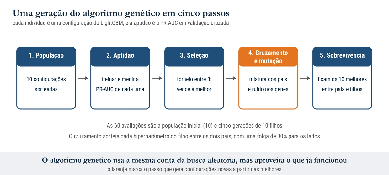
Each individual is a vector of 7 numbers between 0 and 1, which a function converts into the real hyperparameters (with the logarithmic scale where it applies). This makes crossover and mutation independent of each parameter's units.
def genetico(obj, n, semente, populacao=10, torneio=3, p_cruz=0.8, alfa=0.3, p_mut=0.2, sigma=0.12):
    rng = np.random.default_rng(semente)
    d = len(NOMES)
    hist = []

    def avaliar(u):
        p = de_unitario(u)
        s = obj(p)
        hist.append((p, s))
        return s

    pop = [rng.random(d) for _ in range(populacao)]
    fit = [avaliar(u) for u in pop]
    while len(hist) < n:
        filhos = []
        while len(filhos) < populacao and len(hist) + len(filhos) < n:
            def escolher():
                idx = rng.choice(len(pop), torneio, replace=False)
                return pop[max(idx, key=lambda i: fit[i])]
            a, b = escolher(), escolher()
            if rng.random() < p_cruz:
                lo, hi = np.minimum(a, b), np.maximum(a, b)
                amp = hi - lo
                filho = rng.uniform(lo - alfa * amp, hi + alfa * amp)
            else:
                filho = a.copy()
            mut = rng.random(d) < p_mut
            filho = np.clip(filho + mut * rng.normal(0, sigma, d), 0, 1)
            filhos.append(filho)
        fit_f = [avaliar(u) for u in filhos]
        todos, fits = pop + filhos, fit + fit_f
        ordem = np.argsort(fits)[::-1][:populacao]
        pop, fit = [todos[i] for i in ordem], [fits[i] for i in ordem]
    return hist
With 60 evaluations, the genetic algorithm uses the initial population (10) and five generations of 10 children, that is, 10 + 5 × 10 = 60.
Everyone quickly reaches the same place
Figure 2 shows the best validation value found up to evaluation n, averaged over the 10 runs of each method. All 10 runs of each method went above 0.66 validation PR-AUC, well above the default configuration, and the median number of evaluations to pass 0.66 was 2 for the four methods.
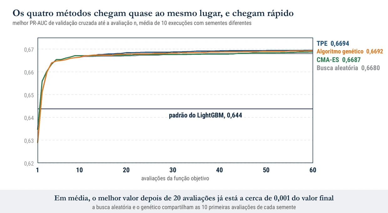
Since one or two draws already pass the default, the search space is generous, and almost any reasonable configuration beats the default. The next 40 evaluations refine little.
| Method | Validation PR-AUC, mean (SD) | Test PR-AUC, mean (SD) | Test, minimum and maximum |
|---|---|---|---|
| TPE (Optuna) | 0.6694 (0.0006) | 0.6629 (0.0024) | 0.6599 to 0.6674 |
| Genetic algorithm | 0.6692 (0.0008) | 0.6618 (0.0019) | 0.6585 to 0.6640 |
| CMA-ES (Optuna) | 0.6687 (0.0010) | 0.6615 (0.0029) | 0.6565 to 0.6662 |
| Random search | 0.6680 (0.0006) | 0.6605 (0.0025) | 0.6562 to 0.6650 |
| LightGBM default | 0.6438 | 0.6338 |
The order is the same in validation and on the test, with TPE in front and random search behind. But the distance between the methods is about the size of the spread between seeds of a single method, and both appear in the table.
On the sealed test
Figure 3 shows the test result of each run. The points of the four methods overlap, and all are above the black line of the default.
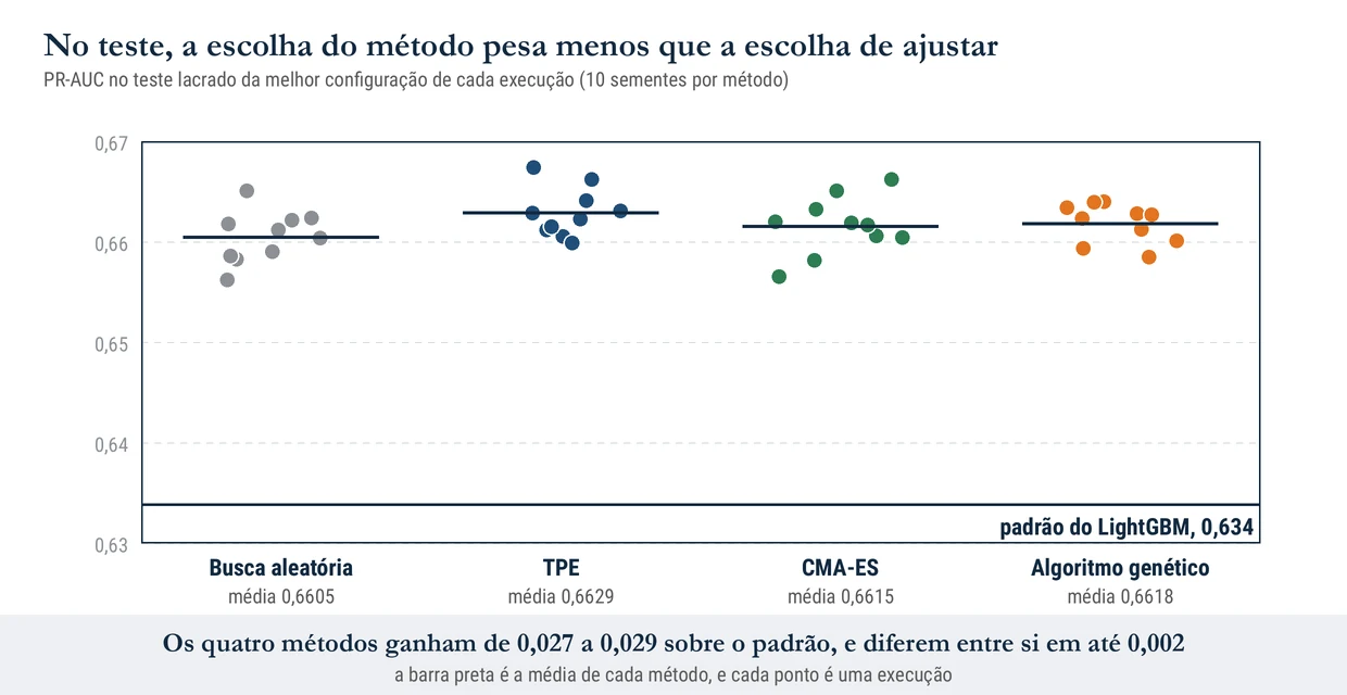
To find out whether the difference from random search is real, I compare each method with it, seed by seed. Then I compute a 95% confidence interval for the mean difference, drawing the seeds with replacement many times (bootstrap). If the interval crosses zero, the difference may be chance.
| Method against random search | Validation, difference (95% CI) | Test, difference (95% CI) |
|---|---|---|
| TPE | +0.0013 (0.0008 to 0.0019) | +0.0024 (0.0002 to 0.0046) |
| Genetic algorithm | +0.0011 (0.0006 to 0.0017) | +0.0013 (-0.0006 to 0.0034) |
| CMA-ES | +0.0006 (-0.0002 to 0.0014) | +0.0011 (-0.0013 to 0.0033) |
In validation, TPE and the genetic algorithm pass random search with the whole interval above zero, but validation is what the methods try to maximize, so it is already a little inflated in their favor.
The test, which the search never saw, is what decides, and there only TPE separates from random search, and barely, because the lower limit of the interval is 0.0002. The genetic algorithm and CMA-ES have a positive difference, but the interval includes zero.
Which method to use, then? For this problem, what we can say is that tuning is worth it and that the method hardly matters. TPE is a good default choice, because it has the highest mean in both measures (validation and test) and already comes ready in Optuna. Random search with 60 evaluations already captures more than 90% of the possible gain (0.0267 of 0.0291 on the test). The genetic algorithm only pays off if you need something the libraries do not offer, such as constraints between hyperparameters or a kind of gene that is not a number.
Where this result does not hold
It is one dataset, one model and a space of 7 hyperparameters, and the result does not hold for other problems. In a larger or more rugged space, such as that of a neural network, the methods that use the history may separate more. The genetic algorithm's hyperparameters (population of 10, tournament of 3, mutation of 0.2) are the ones I chose beforehand, without tuning, and other values could change the order. In the comparison, random search and the genetic algorithm start from the same initial draw.
I did not compare wall-clock time, only the number of objective evaluations, and with fast training like this the cost of the search itself is small. The validation PR-AUC is about 0.007 above the test one in the four methods, and part of that is the search adjusting itself to the objective. Finally, ten seeds give wide intervals, and the differences of 0.001 that appear here are too small to decide anything in production.
For the next search
If I were tuning another model tomorrow, I would start with the default configuration, just to have the reference metric and know how much the tuning pays off. Then I would run 20 to 30 evaluations of random search, which in this problem already capture almost all of the gain. TPE comes in if each evaluation costs hours, and the genetic algorithm is left for when what you are searching for is not a vector of numbers, like the order in which boxes go into a truck, which is the subject of the article on cargo load optimization with a genetic algorithm.
And before comparing two methods, several seeds. A single pretty run can be just luck.
References
BERGSTRA, James; BENGIO, Yoshua. Random search for hyper-parameter optimization. Journal of Machine Learning Research, v. 13, p. 281-305, 2012.
AKIBA, Takuya; SANO, Shotaro; YANASE, Toshihiko; OHTA, Takeru; KOYAMA, Masanori. Optuna: a next-generation hyperparameter optimization framework. In: ACM SIGKDD International Conference on Knowledge Discovery and Data Mining, 25., 2019. DOI: 10.1145/3292500.3330701


