Estimating Deep Learning Project Duration with Simulation and Markov Chains

One of the big problems when training artificial intelligence models is that we are often working very close to the edge of the state of the art of a new technique, and yet we frequently have to estimate how much time we would need to train a model and get it into production.

To train a model, however, many steps are carried out, and they are often repeated until we reach the expected result, assuming, of course, that you go through all the steps of scoping the research and so on.

The usual steps of this work are divided into Sample, Training, Validation and Production. They are often mistaken for a linear sequence of procedures, but they are actually part of a very complex network, which can be understood as a network of connected stages, each with a probability of moving forward or returning to the same stage.

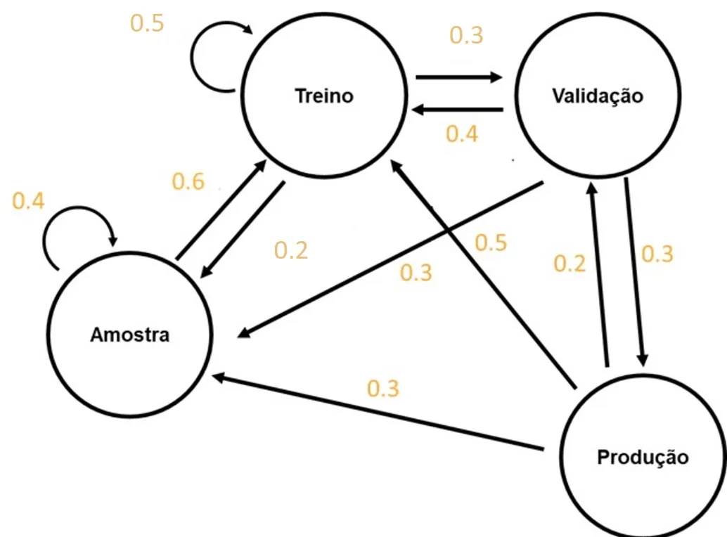
This way, we can make an estimate using the Markov chain method.

For the work here, we only need to import four python libraries.

import numpy as np 
import random as rm 
import pandas as pd 
import matplotlib.pyplot as plt

We start the graph problem by defining the model training states.

estados_desenvolvimento = ["Amostra", "Treino", "Validação","Produção"]

Followed by the matrix of possible sequences...

sequencias = [["Amostra -> Amostra", "Amostra -> Treino",
               "Amostra -> Validação", "Amostra -> Produção"],
               ["Treino -> Amostra", "Treino -> Treino",
               "Treino -> Validação", "Treino -> Produção"],
               ["Validação -> Amostra", "Validação -> Treino",
               "Validação -> Validação", "Validação -> Produção"],
               ["Produção -> Amostra", "Produção -> Treino",
               "Produção -> Validação", "Produção -> Produção"]]

And the state transition probabilities. These probabilities were defined through a somewhat qualitative discussion of the difficulties of the process; if you want to replicate this and have the information, I recommend using real data.

prob_sequencia = [[0.4, 0.6, 0.0, 0.0],
                  [0.2, 0.5, 0.3, 0.0],
                  [0.3, 0.4, 0.0, 0.3],
                  [0.3, 0.5, 0.2, 0.0]]

The functions I created for this work can be found in the Notebook. I won't dwell on the code, but rather on the method and the results.

With the probabilities, we can estimate the next state in the sequence, starting from the initial state "Amostra" (Sample).

estato_atual = 'Amostra'

atividades_modelo.next_state(current_state = estato_atual)

>>> "Treino"

So, if we assume that each state transition takes 1 week, we can run simulations over a given number of weeks.

numero_semanas  = 10

resultado = atividades_modelo.generate_states(current_state = estato_atual, no = numero_semanas)

>>> ['Treino', 'Validação', 'Treino', 'Validação', 'Treino', 'Amostra',
 'Treino', 'Treino', m'Validação', 'Amostra']

We can also define the final state at which we want to end our simulation. In this case, as with any model, we want to put it into production.

estato_futuro = 'Produção'

resultado = atividades_modelo.generate_especific_states(current_state = estato_atual, stop_state = estato_futuro )

>>> ['Treino', 'Amostra', 'Treino', 'Treino', 'Amostra', 'Treino',
 'Validação','Amostra', 'Treino', 'Treino', 'Amostra', 'Treino', 
 'Amostra', 'Treino', 'Treino', 'Amostra', 'Amostra', 'Amostra',
 'Treino', 'Treino', 'Treino', 'Treino', 'Amostra', 'Treino',
 'Amostra', 'Amostra', 'Amostra', 'Treino', 'Treino', 'Treino',
 'Treino', 'Validação', 'Produção']

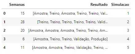
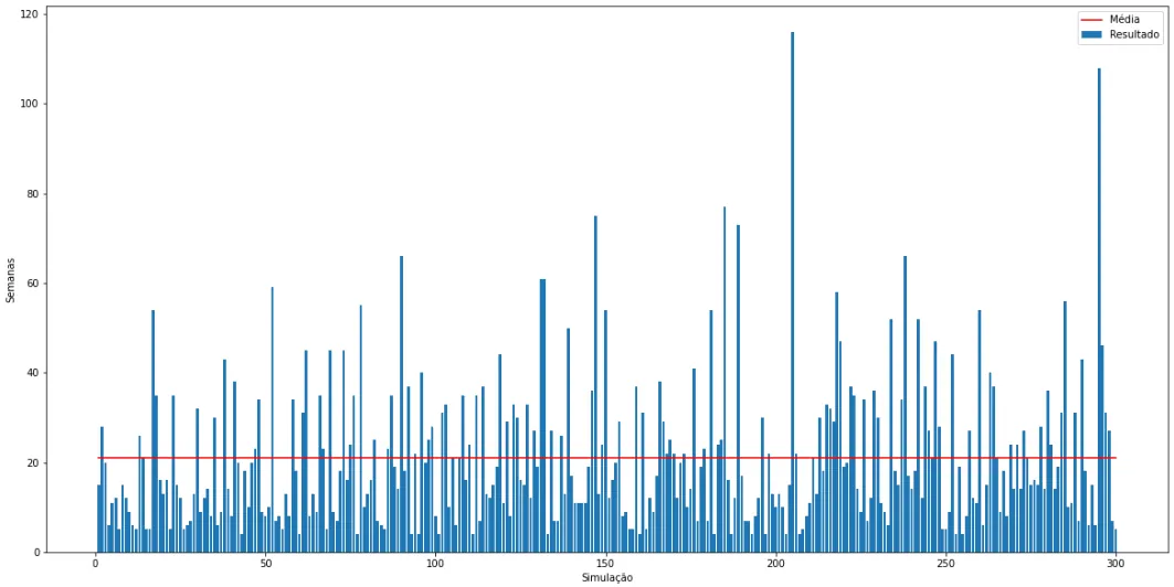
Having reached a given final state, we can repeat this operation many times and thus determine, for example, the average time needed to train the models, which in this case was 21 weeks.

In addition, we can analyze the simulation results graphically and identify the maximum time any of these simulations could take, which in this case was 118 weeks.

With this, we can set the time limits for delivering the work, with a maximum of, in this case, 16 weeks (4 months) and a minimum of 4 weeks (1 complete cycle from training to production).

simulacoes = 300
semana_maxima = 16
semana_min = 4

resultado = atividades_modelo.generate_risc(current_state = estato_atual,                                             stop_state = estato_futuro, nn = semana_min, nm = semana_maxima,  sm = simulacoes )

print(f"Dá Errado {round(resultado[3],2)} % \nDá Certo {round(resultado[4],2)} %")

>>> 
Dá Errado 52.67 % 
Dá Certo 47.33 %

So, based on the stage probabilities for training a deep learning model with a maximum delivery deadline of 16 weeks, we can conclude that there is a 52.67% chance of exceeding the schedule's time limit.

Given that the 16-week maximum cannot be changed, we can instead change other variables, such as the stage transition probabilities. One example would be reducing the probabilities of the Training -> Sample and Training -> Training cycles. These improvements could come from image processing, building on the work already done, or from improving the performance of the machine running the training, shrinking the time scale so that a training run does not take a whole week.