Customer Churn Prediction for Telecom Companies

Translated from the original Portuguese article. Ler o original em português


Telecommunications service providers routinely analyze customer dissatisfaction, always tracking whether their customers are satisfied or not. These analyses are among the key metrics for retaining customers and acquiring new ones. Companies in this sector usually have customer service departments, and one of their main tasks is trying to win back lost customers, who can cost much more than new ones.
Because of this, companies invest in new technologies to carry out these analyses, commonly relying on the Churn rate, or simply Churn, one of the ways to measure customer attrition. Besides measuring this attrition rate, Churn analysis helps anticipate future cancellations, producing predictions that support decision-making and targeted actions for these customers. A familiar everyday example is streaming companies such as Spotify and Netflix.
Because it is such an important metric, Carlos Melo, in his Data Science na Prática course, gave us a challenge: implement a churn solution from scratch for a telecommunications company using real data. The data used in this project was originally made available on the IBM Developer learning platform. It represents a typical problem faced by telecom companies, and the full dataset can be found at this link.
The data provided by IBM doesn't come with explicit documentation, but fortunately the column names make the problem easy to understand, as we can see in the first five entries below, from a dataset of 7043 entries and 21 columns.
| customerID | gender | SeniorCitizen | Partner | Dependents | tenure | PhoneService | MultipleLines | InternetService | OnlineSecurity | OnlineBackup | DeviceProtection | TechSupport | StreamingTV | StreamingMovies | Contract | PaperlessBilling | PaymentMethod | MonthlyCharges | TotalCharges | Churn | |
|---|---|---|---|---|---|---|---|---|---|---|---|---|---|---|---|---|---|---|---|---|---|
| 0 | 7590-VHVEG | Female | 0 | Yes | No | 1 | No | No phone service | DSL | No | Yes | No | No | No | No | Month-to-month | Yes | Electronic check | 29.85 | 29.85 | No |
| 1 | 5575-GNVDE | Male | 0 | No | No | 34 | Yes | No | DSL | Yes | No | Yes | No | No | No | One year | No | Mailed check | 56.95 | 1889.5 | No |
| 2 | 3668-QPYBK | Male | 0 | No | No | 2 | Yes | No | DSL | Yes | Yes | No | No | No | No | Month-to-month | Yes | Mailed check | 53.85 | 108.15 | Yes |
| 3 | 7795-CFOCW | Male | 0 | No | No | 45 | No | No phone service | DSL | Yes | No | Yes | Yes | No | No | One year | No | Bank transfer (automatic) | 42.30 | 1840.75 | No |
| 4 | 9237-HQITU | Female | 0 | No | No | 2 | Yes | No | Fiber optic | No | No | No | No | No | No | Month-to-month | Yes | Electronic check | 70.70 | 151.65 | Yes |
As the first step of any Data Science project, a good exploratory analysis is essential. So I ran the analyses I considered most important, starting with an assessment of the unique values.
This assessment showed that most of the columns in question have more than two categories, which means some processing is needed later on before feeding the model. Other checks were also necessary, such as identifying outliers, computing descriptive statistics, and checking for bias.
| SeniorCitizen | tenure | MonthlyCharges | TotalCharges | |
|---|---|---|---|---|
| count | 7043.000000 | 7043.000000 | 7043.000000 | 7043.000000 |
| mean | 0.162147 | 32.371149 | 64.761692 | 2281.916928 |
| std | 0.368612 | 24.559481 | 30.090047 | 2265.270398 |
| min | 0.000000 | 0.000000 | 18.250000 | 18.800000 |
| 25% | 0.000000 | 9.000000 | 35.500000 | 402.225000 |
| 50% | 0.000000 | 29.000000 | 70.350000 | 1397.475000 |
| 75% | 0.000000 | 55.000000 | 89.850000 | 3786.600000 |
| max | 1.000000 | 72.000000 | 118.750000 | 8684.800000 |
However, the descriptive statistics and the outlier check didn't reveal much. So I took a closer look at the Tenure column, which represents how long each customer has used the service and can indicate "service loyalty". I assumed that the time unit of Tenure is months.
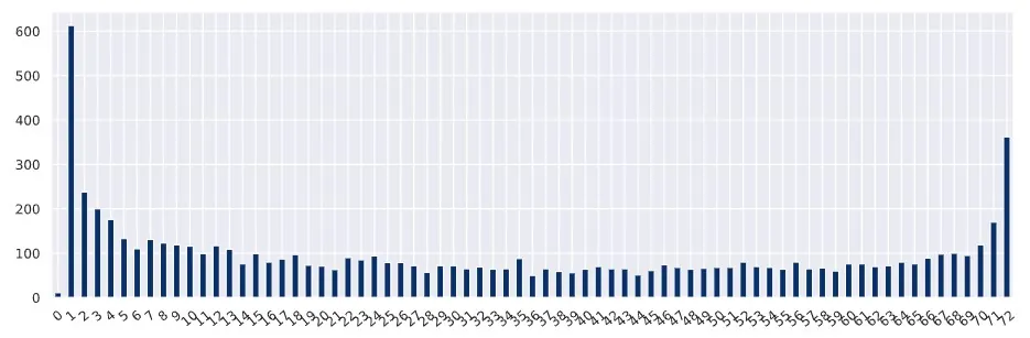
Note that tenure drops from the first month onward, rises again in the last months (70 to 72), but otherwise the data looks fairly regular. Of all the checks mentioned above, I'll highlight the presence of bias, since the others didn't show anything that could compromise the model.
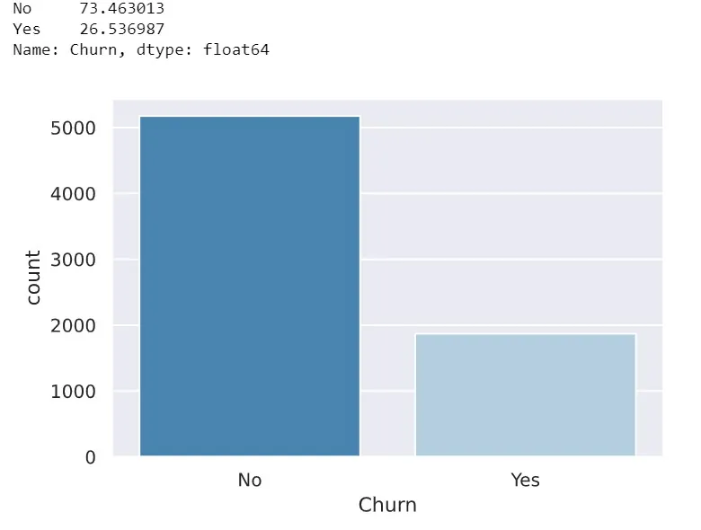
The bias analysis covered the gender, Partner and Churn columns. However, only the last one showed a problematic imbalance, so it had to be balanced, as you can see below:
As for the other columns, some of their unique values could be treated as the same thing, especially in the service columns. Even though this assumption is perfectly valid, in this work I'll keep them as separate values.
At this stage I performed some transformations to prepare the data for building a good model. First came the preprocessing, using LabelEncoder and get_dummies to convert the data into binary variables, putting each class in its own column with a distinct numeric value, as shown below:
| gender | SeniorCitizen | Partner | Dependents | tenure | PhoneService | PaperlessBilling | MonthlyCharges | TotalCharges | Churn | MultipleLines_No | MultipleLines_No phone service | MultipleLines_Yes | InternetService_DSL | InternetService_Fiber optic | InternetService_No | OnlineSecurity_No | OnlineSecurity_No internet service | OnlineSecurity_Yes | OnlineBackup_No | OnlineBackup_No internet service | OnlineBackup_Yes | DeviceProtection_No | DeviceProtection_No internet service | DeviceProtection_Yes | TechSupport_No | TechSupport_No internet service | TechSupport_Yes | StreamingTV_No | StreamingTV_No internet service | StreamingTV_Yes | StreamingMovies_No | StreamingMovies_No internet service | StreamingMovies_Yes | Contract_Month-to-month | Contract_One year | Contract_Two year | PaymentMethod_Bank transfer (automatic) | PaymentMethod_Credit card (automatic) | PaymentMethod_Electronic check | PaymentMethod_Mailed check | |
|---|---|---|---|---|---|---|---|---|---|---|---|---|---|---|---|---|---|---|---|---|---|---|---|---|---|---|---|---|---|---|---|---|---|---|---|---|---|---|---|---|---|
| 0 | 0 | 0 | 1 | 0 | 1 | 0 | 1 | 29.85 | 29.85 | 0 | 0 | 1 | 0 | 1 | 0 | 0 | 1 | 0 | 0 | 0 | 0 | 1 | 1 | 0 | 0 | 1 | 0 | 0 | 1 | 0 | 0 | 1 | 0 | 0 | 1 | 0 | 0 | 0 | 0 | 1 | 0 |
| 1 | 1 | 0 | 0 | 0 | 34 | 1 | 0 | 56.95 | 1889.50 | 0 | 1 | 0 | 0 | 1 | 0 | 0 | 0 | 0 | 1 | 1 | 0 | 0 | 0 | 0 | 1 | 1 | 0 | 0 | 1 | 0 | 0 | 1 | 0 | 0 | 0 | 1 | 0 | 0 | 0 | 0 | 1 |
| 2 | 1 | 0 | 0 | 0 | 2 | 1 | 1 | 53.85 | 108.15 | 1 | 1 | 0 | 0 | 1 | 0 | 0 | 0 | 0 | 1 | 0 | 0 | 1 | 1 | 0 | 0 | 1 | 0 | 0 | 1 | 0 | 0 | 1 | 0 | 0 | 1 | 0 | 0 | 0 | 0 | 0 | 1 |
| 3 | 1 | 0 | 0 | 0 | 45 | 0 | 0 | 42.30 | 1840.75 | 0 | 0 | 1 | 0 | 1 | 0 | 0 | 0 | 0 | 1 | 1 | 0 | 0 | 0 | 0 | 1 | 0 | 0 | 1 | 1 | 0 | 0 | 1 | 0 | 0 | 0 | 1 | 0 | 1 | 0 | 0 | 0 |
| 4 | 0 | 0 | 0 | 0 | 2 | 1 | 1 | 70.70 | 151.65 | 1 | 1 | 0 | 0 | 0 | 1 | 0 | 1 | 0 | 0 | 1 | 0 | 0 | 1 | 0 | 0 | 1 | 0 | 0 | 1 | 0 | 0 | 1 | 0 | 0 | 1 | 0 | 0 | 0 | 0 | 1 | 0 |
With that, we can generate the correlation matrix of the data.
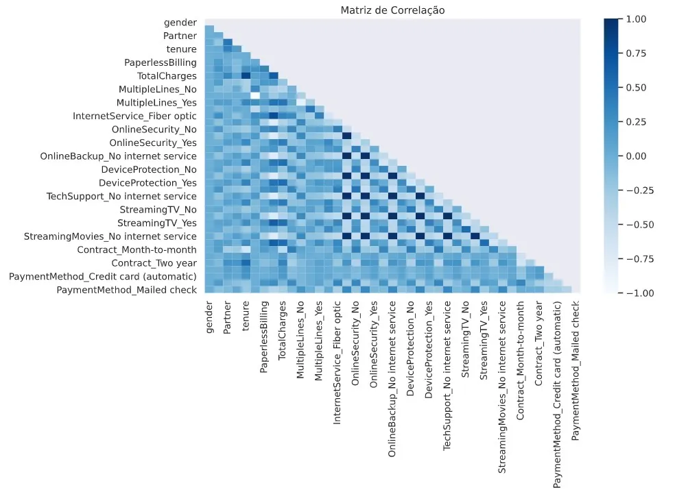
With all of this done, we can move on to the preprocessing and define our performance metric. For error estimation I used Cross-Validation, which I've already discussed in another article, combined with the recall metric to find the best model for this problem.
To make model evaluation easier, I defined a validation function:
#Função de validação

def valid(X, y, model, quite = False):

  X = np.array(X)
  y = np.array(y)
  pipeline = make_pipeline(StandardScaler(), model)
  scores = cross_val_score(pipeline, X, y, scoring="recall")

  if quite == False:
     print("Recall: {:.3f} (+/- {:.3f})".format(scores.mean(), scores.std()))

  return scores.mean()
It returns the recall value and the score. I then built a comparison baseline to serve as a reference for evaluating the models I used.
#Criando linha base
rfc = RandomForestClassifier()
score_baseline = valid(X_treino, y_treino, rfc)
This resulted in Recall: 0.485 (+/- 0.022). The balancing technique was based on Under Sampling, and, following recommendations from the literature, the data is standardized before applying it, and only on the training set.
Since I didn't know which model would perform best, I ran cross-validation for the following models:
- Random Forest
- Decision Trees
- Stochastic Gradient Descent
- SVC
- Logistic Regression
- LightGBM
I then instantiated and configured them as shown below:
#Instanciar os modelos
rc = RandomForestClassifier()
ad = DecisionTreeClassifier()
gde = SGDClassifier()
svc = SVC()
rl = LogisticRegression()
xgb = XGBClassifier()
lgbm = LGBMClassifier()
#Criar lista para resultados
modelo = []
recall = []
#Avaliar desempenho
for clf in (rc, ad, gde, svc, rl, xgb, lgbm):
  modelo.append(clf.__class__.__name__)
  recall.append(valid(X_treino_rus, y_treino_rus, clf, quite = True))

Recall = pd.DataFrame(data = recall, index=modelo, columns=["Recall"])
This produced the following results:
| Recall | |
|---|---|
| LogisticRegression | 0.803375 |
| SVC | 0.793548 |
| XGBClassifier | 0.792170 |
| LGBMClassifier | 0.769701 |
| RandomForestClassifier | 0.752854 |
| SGDClassifier | 0.707198 |
| DecisionTreeClassifier | 0.701591 |
As the results show, XGBoost, Logistic Regression and SVC stood out, all with their default settings. So I took the best model from the previous step (XGBoost) and tuned its parameters to get the best possible result; you can find this in the full project.
After evaluating a few XGBoost configurations, I found the best result to be:
#Modelo Final
xgb=XGBClassifier(learning_rate=0.001,n_estimators=50,max_depth=1,min_child_weight=1,gamma=0.0)xgb.fit(X_treino_rus,y_treino_rus)
XGBClassifier(base_score=0.5, booster='gbtree', colsample_bylevel=1,
              colsample_bynode=1, colsample_bytree=1, gamma=0.0,
              learning_rate=0.001, max_delta_step=0, max_depth=1,
              min_child_weight=1, missing=None, n_estimators=50, n_jobs=1,
              nthread=None, objective='binary:logistic', random_state=0,
              reg_alpha=0, reg_lambda=1, scale_pos_weight=1, seed=None,
              silent=None, subsample=1, verbosity=1)
This gave the following prediction results:
              precision    recall  f1-score   support

           0       0.94      0.57      0.71      1316
           1       0.41      0.89      0.56       445

    accuracy                           0.65      1761
   macro avg       0.67      0.73      0.64      1761
weighted avg       0.80      0.65      0.67      1761

Área sobre a curva ASC: 0.7284109149277687
And the confusion matrix:
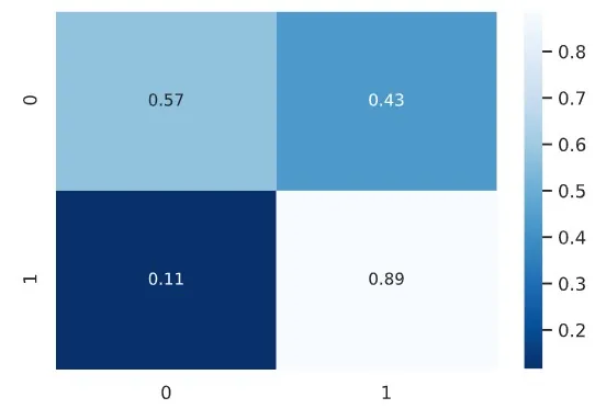
The result is an excellent model, with a true positive rate of 0.89 and a true negative rate of 0.57, and an AUC of 0.72.
In this project, we worked on a churn prediction problem whose main goal was to build a machine learning model capable of correctly identifying as many likely churners as possible. To get there, several steps were needed, such as balancing and standardization, and several models were tested to find the best result, finally arriving at an XGBoost model with an excellent result.