Credit Card Fraud Detection

Translated from the original Portuguese article. Ler o original em português


Credit card fraud is one of the main concerns of financial institutions. In Brazil, around 12 million people have already been victims of fraud, with losses exceeding R$ 1.8 billion in 2019 alone.
However, undetected fraud should not be a concern for financial institutions only, since this problem can cause major losses that reach other financial sectors and even consumers. Because of this, numerous techniques are used to detect fraud, which raises concerns such as false positives, which embarrass countless users when their card is declined and blocked while making a purchase.
There is growing investment in Artificial Intelligence applications, and with large volumes of data as a historical base, a machine learning algorithm that is only slightly better than the previous ones already represents savings of millions of reais. So, as a hands-on exercise of Carlos Melo's Data Science na Prática course, we were challenged to keep improving the use of algorithms to inhibit or prevent fraudulent transactions. Since this is a challenge, Carlos provided the data already organized and without categorical variables, so that this work could focus on building the best possible model.
The data in question was made available by some European credit card companies and represents the financial operations that took place over a two-day period, during which 290 thousand transactions were recorded.
A nice thing about this dataset is that its features are all numeric and anonymized (to protect the users). So the columns are represented as V1, V2 ... V28, and the remaining columns represent the following:
- Time - Number of seconds elapsed between this transaction and the first transaction in the dataset;
- Amount - Transaction amount;
- Class - 1 for fraudulent transactions, 0 otherwise.
As we can see in the first and last five entries.
First entries
| Time | V1 | V2 | V3 | V4 | V5 | V6 | V7 | V8 | V9 | V10 | V11 | V12 | V13 | V14 | V15 | V16 | V17 | V18 | V19 | V20 | V21 | V22 | V23 | V24 | V25 | V26 | V27 | V28 | Amount | Class | |
|---|---|---|---|---|---|---|---|---|---|---|---|---|---|---|---|---|---|---|---|---|---|---|---|---|---|---|---|---|---|---|---|
| 0 | 0.0 | -1.359807 | -0.072781 | 2.536347 | 1.378155 | -0.338321 | 0.462388 | 0.239599 | 0.098698 | 0.363787 | 0.090794 | -0.551600 | -0.617801 | -0.991390 | -0.311169 | 1.468177 | -0.470401 | 0.207971 | 0.025791 | 0.403993 | 0.251412 | -0.018307 | 0.277838 | -0.110474 | 0.066928 | 0.128539 | -0.189115 | 0.133558 | -0.021053 | 149.62 | 0 |
| 1 | 0.0 | 1.191857 | 0.266151 | 0.166480 | 0.448154 | 0.060018 | -0.082361 | -0.078803 | 0.085102 | -0.255425 | -0.166974 | 1.612727 | 1.065235 | 0.489095 | -0.143772 | 0.635558 | 0.463917 | -0.114805 | -0.183361 | -0.145783 | -0.069083 | -0.225775 | -0.638672 | 0.101288 | -0.339846 | 0.167170 | 0.125895 | -0.008983 | 0.014724 | 2.69 | 0 |
| 2 | 1.0 | -1.358354 | -1.340163 | 1.773209 | 0.379780 | -0.503198 | 1.800499 | 0.791461 | 0.247676 | -1.514654 | 0.207643 | 0.624501 | 0.066084 | 0.717293 | -0.165946 | 2.345865 | -2.890083 | 1.109969 | -0.121359 | -2.261857 | 0.524980 | 0.247998 | 0.771679 | 0.909412 | -0.689281 | -0.327642 | -0.139097 | -0.055353 | -0.059752 | 378.66 | 0 |
| 3 | 1.0 | -0.966272 | -0.185226 | 1.792993 | -0.863291 | -0.010309 | 1.247203 | 0.237609 | 0.377436 | -1.387024 | -0.054952 | -0.226487 | 0.178228 | 0.507757 | -0.287924 | -0.631418 | -1.059647 | -0.684093 | 1.965775 | -1.232622 | -0.208038 | -0.108300 | 0.005274 | -0.190321 | -1.175575 | 0.647376 | -0.221929 | 0.062723 | 0.061458 | 123.50 | 0 |
| 4 | 2.0 | -1.158233 | 0.877737 | 1.548718 | 0.403034 | -0.407193 | 0.095921 | 0.592941 | -0.270533 | 0.817739 | 0.753074 | -0.822843 | 0.538196 | 1.345852 | -1.119670 | 0.175121 | -0.451449 | -0.237033 | -0.038195 | 0.803487 | 0.408542 | -0.009431 | 0.798278 | -0.137458 | 0.141267 | -0.206010 | 0.502292 | 0.219422 | 0.215153 | 69.99 | 0 |
Last entries
| Time | V1 | V2 | V3 | V4 | V5 | V6 | V7 | V8 | V9 | V10 | V11 | V12 | V13 | V14 | V15 | V16 | V17 | V18 | V19 | V20 | V21 | V22 | V23 | V24 | V25 | V26 | V27 | V28 | Amount | Class | |
|---|---|---|---|---|---|---|---|---|---|---|---|---|---|---|---|---|---|---|---|---|---|---|---|---|---|---|---|---|---|---|---|
| 284802 | 172786.0 | -11.881118 | 10.071785 | -9.834783 | -2.066656 | -5.364473 | -2.606837 | -4.918215 | 7.305334 | 1.914428 | 4.356170 | -1.593105 | 2.711941 | -0.689256 | 4.626942 | -0.924459 | 1.107641 | 1.991691 | 0.510632 | -0.682920 | 1.475829 | 0.213454 | 0.111864 | 1.014480 | -0.509348 | 1.436807 | 0.250034 | 0.943651 | 0.823731 | 0.77 | 0 |
| 284803 | 172787.0 | -0.732789 | -0.055080 | 2.035030 | -0.738589 | 0.868229 | 1.058415 | 0.024330 | 0.294869 | 0.584800 | -0.975926 | -0.150189 | 0.915802 | 1.214756 | -0.675143 | 1.164931 | -0.711757 | -0.025693 | -1.221179 | -1.545556 | 0.059616 | 0.214205 | 0.924384 | 0.012463 | -1.016226 | -0.606624 | -0.395255 | 0.068472 | -0.053527 | 24.79 | 0 |
| 284804 | 172788.0 | 1.919565 | -0.301254 | -3.249640 | -0.557828 | 2.630515 | 3.031260 | -0.296827 | 0.708417 | 0.432454 | -0.484782 | 0.411614 | 0.063119 | -0.183699 | -0.510602 | 1.329284 | 0.140716 | 0.313502 | 0.395652 | -0.577252 | 0.001396 | 0.232045 | 0.578229 | -0.037501 | 0.640134 | 0.265745 | -0.087371 | 0.004455 | -0.026561 | 67.88 | 0 |
| 284805 | 172788.0 | -0.240440 | 0.530483 | 0.702510 | 0.689799 | -0.377961 | 0.623708 | -0.686180 | 0.679145 | 0.392087 | -0.399126 | -1.933849 | -0.962886 | -1.042082 | 0.449624 | 1.962563 | -0.608577 | 0.509928 | 1.113981 | 2.897849 | 0.127434 | 0.265245 | 0.800049 | -0.163298 | 0.123205 | -0.569159 | 0.546668 | 0.108821 | 0.104533 | 10.00 | 0 |
| 284806 | 172792.0 | -0.533413 | -0.189733 | 0.703337 | -0.506271 | -0.012546 | -0.649617 | 1.577006 | -0.414650 | 0.486180 | -0.915427 | -1.040458 | -0.031513 | -0.188093 | -0.084316 | 0.041333 | -0.302620 | -0.660377 | 0.167430 | -0.256117 | 0.382948 | 0.261057 | 0.643078 | 0.376777 | 0.008797 | -0.473649 | -0.818267 | -0.002415 | 0.013649 | 217.00 | 0 |
The original data can be found on Kaggle, and it has been transformed with a technique known as Principal Component Analysis (PCA). This technique reduces dimensionality while retaining as much information as possible. To achieve this, the algorithm finds a new set of features, the so-called components, whose number is less than or equal to that of the original variables.
With the data loaded into a DataFrame structure and no further adjustment or configuration needed at this stage, I was able to go straight to the exploratory data analysis and, finally, to building the Machine Learning model.
I started by analyzing the basic statistics. This is an important part of the work, where we look at the distribution and balance of each column.
| Time | V1 | V2 | V3 | V4 | V5 | V6 | V7 | V8 | V9 | V10 | V11 | V12 | V13 | V14 | V15 | V16 | V17 | V18 | V19 | V20 | V21 | V22 | V23 | V24 | V25 | V26 | V27 | V28 | Amount | Class | |
|---|---|---|---|---|---|---|---|---|---|---|---|---|---|---|---|---|---|---|---|---|---|---|---|---|---|---|---|---|---|---|---|
| count | 284807.000000 | 2.848070e+05 | 2.848070e+05 | 2.848070e+05 | 2.848070e+05 | 2.848070e+05 | 2.848070e+05 | 2.848070e+05 | 2.848070e+05 | 2.848070e+05 | 2.848070e+05 | 2.848070e+05 | 2.848070e+05 | 2.848070e+05 | 2.848070e+05 | 2.848070e+05 | 2.848070e+05 | 2.848070e+05 | 2.848070e+05 | 2.848070e+05 | 2.848070e+05 | 2.848070e+05 | 2.848070e+05 | 2.848070e+05 | 2.848070e+05 | 2.848070e+05 | 2.848070e+05 | 2.848070e+05 | 2.848070e+05 | 284807.000000 | 284807.000000 |
| mean | 94813.859575 | 3.919560e-15 | 5.688174e-16 | -8.769071e-15 | 2.782312e-15 | -1.552563e-15 | 2.010663e-15 | -1.694249e-15 | -1.927028e-16 | -3.137024e-15 | 1.768627e-15 | 9.170318e-16 | -1.810658e-15 | 1.693438e-15 | 1.479045e-15 | 3.482336e-15 | 1.392007e-15 | -7.528491e-16 | 4.328772e-16 | 9.049732e-16 | 5.085503e-16 | 1.537294e-16 | 7.959909e-16 | 5.367590e-16 | 4.458112e-15 | 1.453003e-15 | 1.699104e-15 | -3.660161e-16 | -1.206049e-16 | 88.349619 | 0.001727 |
| std | 47488.145955 | 1.958696e+00 | 1.651309e+00 | 1.516255e+00 | 1.415869e+00 | 1.380247e+00 | 1.332271e+00 | 1.237094e+00 | 1.194353e+00 | 1.098632e+00 | 1.088850e+00 | 1.020713e+00 | 9.992014e-01 | 9.952742e-01 | 9.585956e-01 | 9.153160e-01 | 8.762529e-01 | 8.493371e-01 | 8.381762e-01 | 8.140405e-01 | 7.709250e-01 | 7.345240e-01 | 7.257016e-01 | 6.244603e-01 | 6.056471e-01 | 5.212781e-01 | 4.822270e-01 | 4.036325e-01 | 3.300833e-01 | 250.120109 | 0.041527 |
| min | 0.000000 | -5.640751e+01 | -7.271573e+01 | -4.832559e+01 | -5.683171e+00 | -1.137433e+02 | -2.616051e+01 | -4.355724e+01 | -7.321672e+01 | -1.343407e+01 | -2.458826e+01 | -4.797473e+00 | -1.868371e+01 | -5.791881e+00 | -1.921433e+01 | -4.498945e+00 | -1.412985e+01 | -2.516280e+01 | -9.498746e+00 | -7.213527e+00 | -5.449772e+01 | -3.483038e+01 | -1.093314e+01 | -4.480774e+01 | -2.836627e+00 | -1.029540e+01 | -2.604551e+00 | -2.256568e+01 | -1.543008e+01 | 0.000000 | 0.000000 |
| 25% | 54201.500000 | -9.203734e-01 | -5.985499e-01 | -8.903648e-01 | -8.486401e-01 | -6.915971e-01 | -7.682956e-01 | -5.540759e-01 | -2.086297e-01 | -6.430976e-01 | -5.354257e-01 | -7.624942e-01 | -4.055715e-01 | -6.485393e-01 | -4.255740e-01 | -5.828843e-01 | -4.680368e-01 | -4.837483e-01 | -4.988498e-01 | -4.562989e-01 | -2.117214e-01 | -2.283949e-01 | -5.423504e-01 | -1.618463e-01 | -3.545861e-01 | -3.171451e-01 | -3.269839e-01 | -7.083953e-02 | -5.295979e-02 | 5.600000 | 0.000000 |
| 50% | 84692.000000 | 1.810880e-02 | 6.548556e-02 | 1.798463e-01 | -1.984653e-02 | -5.433583e-02 | -2.741871e-01 | 4.010308e-02 | 2.235804e-02 | -5.142873e-02 | -9.291738e-02 | -3.275735e-02 | 1.400326e-01 | -1.356806e-02 | 5.060132e-02 | 4.807155e-02 | 6.641332e-02 | -6.567575e-02 | -3.636312e-03 | 3.734823e-03 | -6.248109e-02 | -2.945017e-02 | 6.781943e-03 | -1.119293e-02 | 4.097606e-02 | 1.659350e-02 | -5.213911e-02 | 1.342146e-03 | 1.124383e-02 | 22.000000 | 0.000000 |
| 75% | 139320.500000 | 1.315642e+00 | 8.037239e-01 | 1.027196e+00 | 7.433413e-01 | 6.119264e-01 | 3.985649e-01 | 5.704361e-01 | 3.273459e-01 | 5.971390e-01 | 4.539234e-01 | 7.395934e-01 | 6.182380e-01 | 6.625050e-01 | 4.931498e-01 | 6.488208e-01 | 5.232963e-01 | 3.996750e-01 | 5.008067e-01 | 4.589494e-01 | 1.330408e-01 | 1.863772e-01 | 5.285536e-01 | 1.476421e-01 | 4.395266e-01 | 3.507156e-01 | 2.409522e-01 | 9.104512e-02 | 7.827995e-02 | 77.165000 | 0.000000 |
| max | 172792.000000 | 2.454930e+00 | 2.205773e+01 | 9.382558e+00 | 1.687534e+01 | 3.480167e+01 | 7.330163e+01 | 1.205895e+02 | 2.000721e+01 | 1.559499e+01 | 2.374514e+01 | 1.201891e+01 | 7.848392e+00 | 7.126883e+00 | 1.052677e+01 | 8.877742e+00 | 1.731511e+01 | 9.253526e+00 | 5.041069e+00 | 5.591971e+00 | 3.942090e+01 | 2.720284e+01 | 1.050309e+01 | 2.252841e+01 | 4.584549e+00 | 7.519589e+00 | 3.517346e+00 | 3.161220e+01 | 3.384781e+01 | 25691.160000 | 1.000000 |
However, since this is a large dataset, the basic statistics do not convey much information, except that the data shows imbalanced distributions, which we will look at further ahead.
Before that, the next step checked the quality of the dataset, an important metric that tells us whether we can move forward with the project. When computing missing values, none were found.
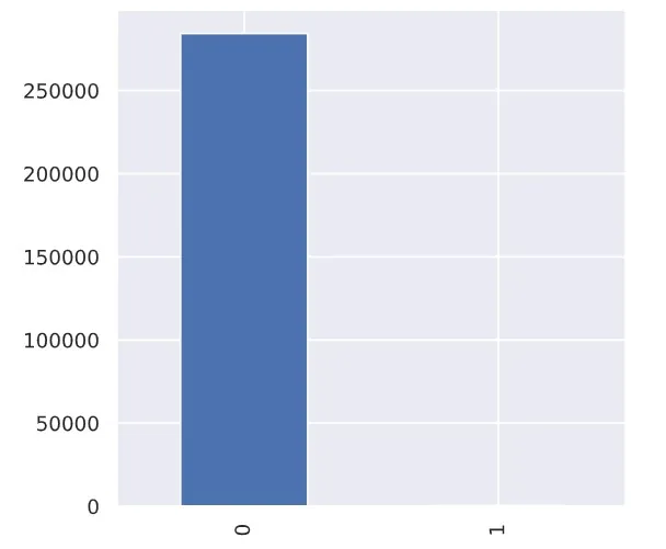
Then I began evaluating the class balance: 0 (Non-fraudulent) with 284,315 entries and 1 (Fraudulent) with 492. Both graphically and in percentage terms, it was clear that the number of fraudulent transactions is much smaller than the number of normal ones, accounting for only 0.17% of the entire dataset.
Next, I created histograms of the two classes with different scales, plotting Time for each Class.
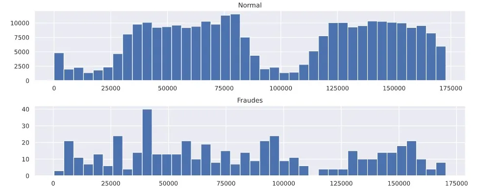
However, it was not possible to extract any information from these two frequency distributions. So I plotted histograms of the classes with respect to Amount.
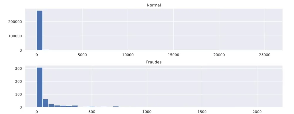
For this data, the histogram distributions show an imbalance and a large presence of possible outliers. So we need to evaluate them with a boxplot for a more in-depth analysis.
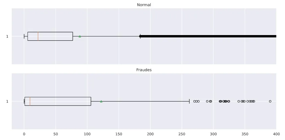
The box plot showed many outliers and clearly a very high imbalance, with a mean of 118.13 and a median of 9.21.
With the balance assessment done, I computed the correlation by plotting a correlation matrix, hiding the upper triangle.
#Criando uma máscara da diagonal superior
mask = np.zeros_like(df.corr())
mask[np.triu_indices_from(mask)] = True
#Plotar matriz de correlação
plt.figure(figsize=(10,6))plt.title("Matriz de Correlação")sns.heatmap(df.corr(),mask=mask,cmap='Blues')plt.show()
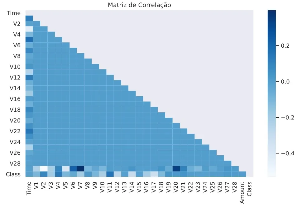
This matrix showed little relationship between the variables, caused by the class imbalance.
To feed the Logistic Regression model we will build, in this preparation step we will:
- Standardize the Time and Amount features, which are on a different order of magnitude.
- Split the data into training and test sets.
- Balance the data to avoid poor performance on class 1 and overfitting.
First I normalized the data, as I have done before here on the blog (link). This technique puts all the model's data on the same scale; in this case I used StandardScaler from the scikit learn library.
#Nomalizar os dados
standert=StandardScaler()X.Time=standert.fit_transform(X.Time.values.reshape(-1,1))X.Amount=standert.fit_transform(X.Amount.values.reshape(-1,1))
After that, I split the data into training and test sets, which made it possible to balance the data using the RandomUnderSampler algorithm from the imblearn library, ending up with 369 entries for each class.
#Balancear os dados
rUS = RandomUnderSampler()
X_rus, y_rus = rUS.fit_sample(X_train, y_train)
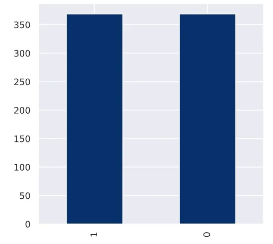
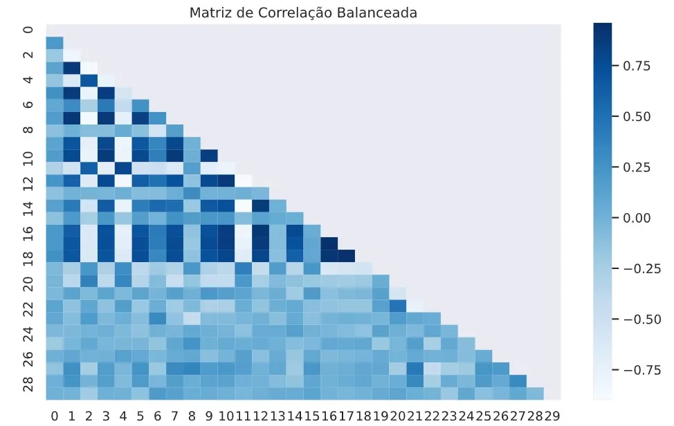
After balancing, I computed the correlation again, and it turned out to be much stronger, showing how important data balancing is when building a good model.
#Criando uma mascara da diagonal superior
mask = np.zeros_like(X_new_df.corr())
mask[np.triu_indices_from(mask)] = True
#Plotar matriz de correlação
plt.figure(figsize = (10,6))
plt.title("Matriz de Correlação Balanceada")

sns.heatmap(X_new_df.corr(), mask= mask, cmap = 'Blues')
plt.show()
With everything ready and a solid exploratory analysis done, we can easily build the Logistic Regression model. This regression model relies on the concept of likelihood, which makes it possible to estimate the probability associated with the occurrence of certain events given a set of explanatory variables.
#Construir modelo de regressão logistica
model = LogisticRegression()
model.fit(X_rus, y_rus)
LogisticRegression(C=1.0, class_weight=None, dual=False, fit_intercept=True,
                   intercept_scaling=1, l1_ratio=None, max_iter=100,
                   multi_class='auto', n_jobs=None, penalty='l2',
                   random_state=None, solver='lbfgs', tol=0.0001, verbose=0,
                   warm_start=False)
With the model trained and the predictions made, I could then analyze its performance. However, in situations like this one, where the data is imbalanced, we cannot use accuracy as a metric. So we need to build a confusion matrix and a classification report.
Relatório de Classificação:               precision    recall  f1-score   support

           0    0.99975   0.96127   0.98013     71079
           1    0.03708   0.86179   0.07109       123

    accuracy                        0.96110     71202
   macro avg    0.51841   0.91153   0.52561     71202
weighted avg    0.99809   0.96110   0.97856     71202
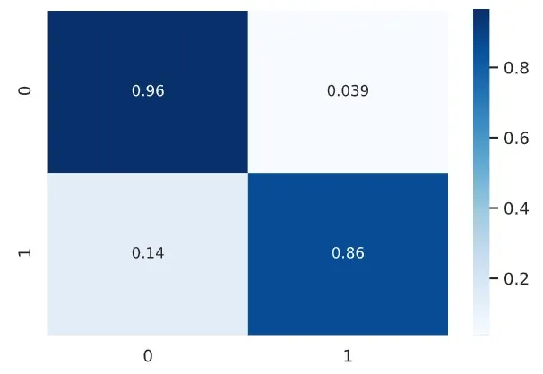
We obtained quite interesting results, with few false negatives and false positives, reaching 96% true negatives and 86% true positives.
Note that this project is not a typical problem: even though it was done with clean, well-prepared data provided by the course instructor, it was necessary to balance and normalize the data and apply PCA before building the model, which then delivered excellent results for the goal at hand. However, this is a didactic project, which had no categorical variables or missing data. That leaves open the gap of building the model with the full Kaggle dataset. You can see the complete project and all the code in my repository.
If you liked it, share it ;)