

Updated 2026 (published in 2021)
Beef cattle prices, female slaughter and the cattle cycle: what 29 years of open data show

Translated from the original Portuguese article. Ler o original em português

In the cattle market people say that female slaughter tells where the price is heading. The logic is that of the cattle cycle. When producers cull more breeding cows, female slaughter rises now, but fewer calves are left in the following years, and cattle become scarcer and more expensive. It sounds reasonable, and I wanted to look at the numbers calmly, in open data, to see what shows up and what does not.
I did a descriptive analysis of 29 years of data, from 1997 to 2026, with the real price of cattle and the share of females in slaughter. In four cycles, each peak of the female share was followed by a price peak 2 to 3 years later. The seasonality of the price, which ranged from -5.9% to +5.7% until 2010, fell to about half after that. It is a reading of the data, and not a proof, and at the end I show that the forecasting test did not separate the effect from chance.
The code is in the blog repository on GitHub, and the data come from a download script.
The data
There are three open sources. The cattle price comes from the Paraná series that IPEADATA publishes (average price received by the farmer, in reais per arroba, monthly). The slaughter by type of herd comes from the Quarterly Animal Slaughter Survey of IBGE, through the SIDRA API. The IPCA inflation index comes from the Central Bank. The most cited price indicator in the market, the CEPEA one, blocks automatic download, so I used the Paraná series as an approximation of the national price.
The price becomes real, deflated by the IPCA and expressed in October 2026 reais. The share of females is the sum of cows and heifers divided by the total of steers, cows, young steers and heifers slaughtered, by quarter.
indice = (1 + ipca / 100).cumprod()
real = preco / indice.reindex(preco.index) * indice.iloc[-1]     # R$ por arroba, a preços de out/2026

base = ab[["Bois", "Vacas", "Novilhos", "Novilhas"]].sum(axis=1)
femeas = (ab.Vacas + ab.Novilhas) / base
The result is 118 quarters of slaughter, from 1997Q1 to 2026Q2, and the monthly price since 1995. The real price went from about R$ 125 per arroba in 1997Q1 to a peak of R$ 403 in 2021Q3, and ends at R$ 347. The share of females went from 24.7% in 2001Q3 to 50.6% in 2025Q2.
The cattle price along the year
Seasonality is the regularity that repeats every year. To measure it in the price, I use the STL decomposition of the logarithm of the monthly real price, which separates the trend, the seasonal part and the remainder. The seasonal effect of each month is how much the price sits above or below what the trend would call for.
stl = STL(np.log(real), period=12, robust=True).fit()
efeito = np.exp(stl.seasonal) - 1        # efeito de cada mês, em fração do preço
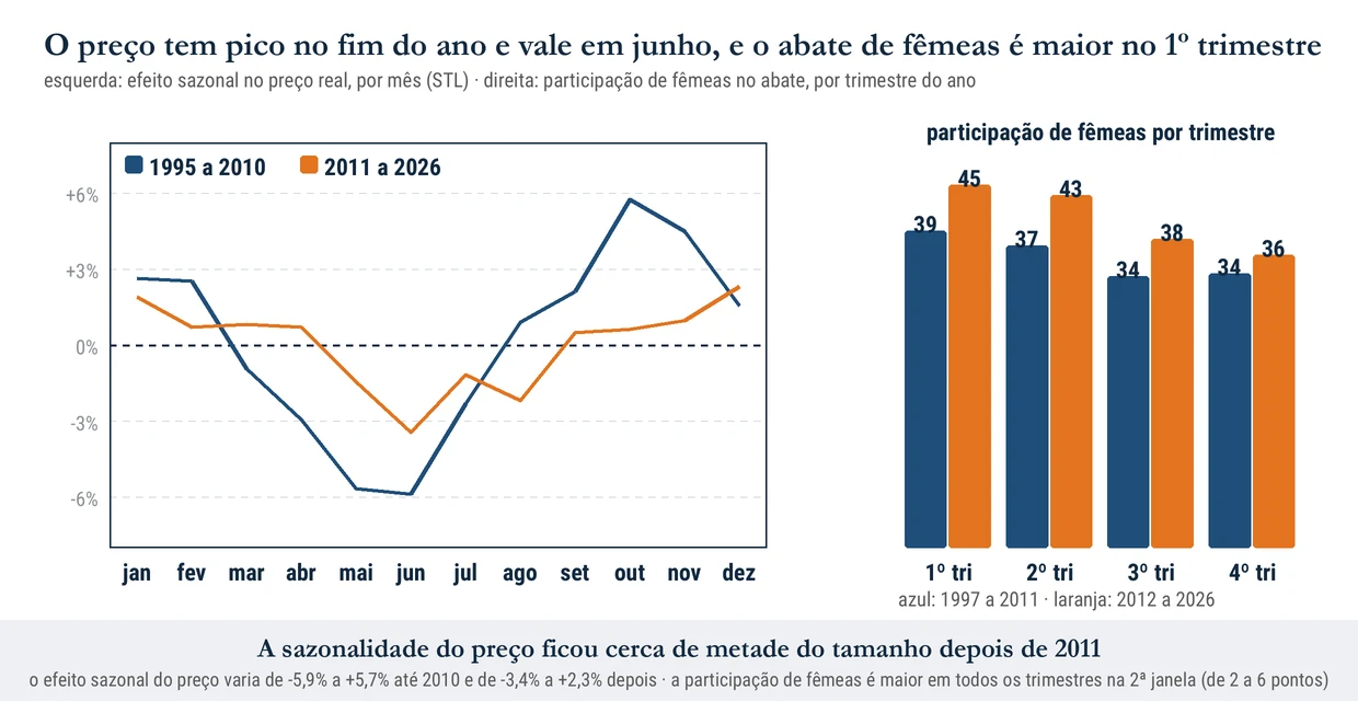
Figure 1 (on the left) shows the pattern in two windows of years. Until 2010 the price was lower from April to July, with the bottom in June (-5.9%), and higher from September to November, with the peak in October (+5.7%). From 2011 on the shape is similar, with the bottom in June (-3.4%), but the peak moves to December (+2.3%) and the amplitude falls from about 11.6 points to about 5.7. Over the 29 years together, the calendar explains little of the price (the seasonal strength, measured after removing the trend, is 0.13 on a scale from 0 to 1), and trend and cycle explain the rest.
A plausible explanation for the drop in amplitude is that the supply of cattle became more constant along the year, for example with more feedlot finishing, but I did not test that.
Female slaughter along the year
In figure 1 (on the right), the share of females by quarter of the year shows that female slaughter is higher in the first quarter and lower in the second half. From 1997 to 2011 it was 39% in the 1st quarter and 34% in the 4th, and from 2012 to 2026 it was 45% and 36%. That means the pattern held, and that the share of females became higher in every quarter in the second window, by 2 to 6 points.
The usual explanation is the culling of females that did not get pregnant, concentrated at the start of the year, and the lower supply of females in the off-season. The data show the pattern, and the explanation I borrow from the market, without having checked it.
The cycle
To see the cycle, I remove the seasonality with a 4-quarter moving average, which covers a whole year and so wipes out the calendar effect. Then I mark the peaks (the highest value in a 4-year window) of the female share and of the price.
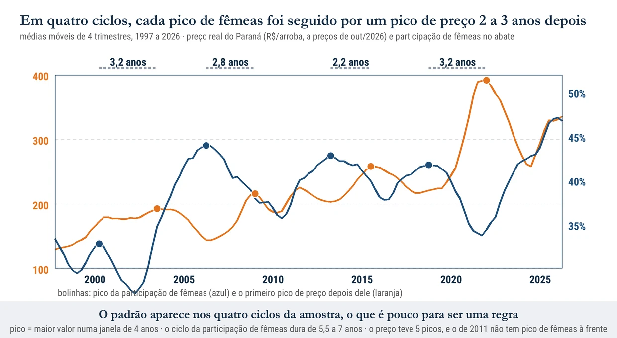
The share of females had peaks in 2000Q2, 2006Q2, 2013Q2 and 2018Q4, so the cycle lasts 5.5 to 7 years (6, 7 and 5.5 years between one peak and the next), which is compatible with the 5 to 6 years the market cites. The real price had peaks in 2003Q3, 2009Q1, 2011Q3, 2015Q3 and 2022Q1. If I take, for each female peak, the first price peak after it, the interval is 3.2 years (2000 to 2003), 2.8 (2006 to 2009), 2.2 (2013 to 2015) and 3.2 (2018 to 2022). It is the pattern of the cycle hypothesis, in four out of four cycles.
Two caveats weigh. The price had five peaks and the share of females, four, so the price peak of 2011 has no female peak ahead of it. And four cycles is few, because a pattern in four cases can appear by chance.
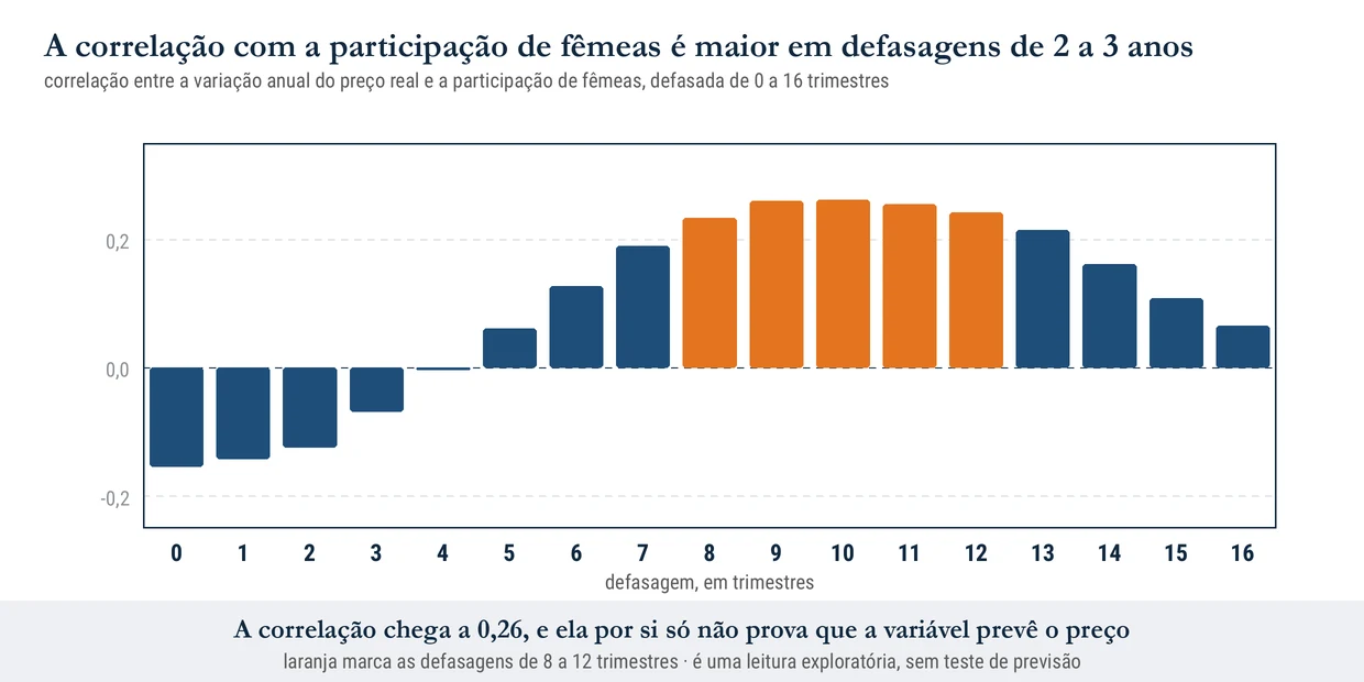
Figure 3 shows the same idea another way, with the correlation between the annual change in the real price and the share of females lagged from 0 to 16 quarters (that is, I compare the price now with the share of females from a few quarters earlier). It is negative at short lags (-0.15 with no lag) and turns positive from 5 quarters, with its highest value, 0.26, at 10 quarters (2.5 years). This agrees with figure 2, because a high share of females now is tied to larger price changes 2 to 3 years later. It is an exploratory reading, and series with trend and cycles can show correlation without one helping to predict the other.
Does it help to forecast?
I tested it. I compared the ARIMA with the price only and the ARIMA with the share of females (and with the dollar), 4 quarters ahead, in 40 rolling origins (40 cutoff dates, and at each one the model uses only the past to forecast the next 4 quarters), using AutoHybTS, an open-source time series library. The error is the mean percentage error. The rule, which I wrote before running, was to accept the hypothesis only if the ARIMA with females made a smaller error in validation, with the confidence interval of the difference entirely below zero, and if the final test did not contradict that result.
The ARIMA with females reduced the validation error by 0.4 percentage point (from 10.1% to 9.7%), but that difference is too small to separate from chance (the confidence interval includes zero). On the 4-quarter test (2025Q3 to 2026Q2, the last year, which I only evaluated at the end) the result did not confirm it either, with the ETS (exponential smoothing) using only the price being the best, with a 1.8% error (it is only 4 quarters, so this number does not compare with the validation ones). By the rule, the forecasting hypothesis was left without support. What the analysis above shows is a pattern of the past, and not a variable that improves forecasting.
So the cycle does not exist? It exists in the data, in the four cycles the sample has. What does not appear is a forecasting improvement that the sample can separate from chance, because there are few cycles to estimate a relation that takes 2 to 3 years to show.
Limits of the reading
The price is the Paraná one, and not the national one, and the share of females is for all of Brazil, so the mismatch between the two can hide or create an effect. Another window for finding the peaks could change the points and the lags. The share of females is a summary of slaughter, and the cycle also depends on the calf price, drought and credit, which do not enter here. The explanations for seasonality and feedlot finishing come from the market, and I did not test them.
The pattern stays, the proof is missing
In 29 years of open data, the real price of cattle has a seasonal bottom in June and a peak at the end of the year, and the share of females is higher in the first quarter. In four cycles, each peak of females was followed by a price peak 2 to 3 years later, but the forecasting test did not separate this from chance.
To say whether the cycle holds, three things are missing, the national price in place of the Paraná one, the calf price and more years of data. Until then, I follow the share of females next to the price, as a context signal, and not as a forecasting variable.
References
INSTITUTO DE PESQUISA ECONÔMICA APLICADA (IPEA). IPEADATA: average price received by the farmer, beef cattle, arroba, Paraná (series DERAL12_PRBGO12). Available at ipeadata.gov.br.
INSTITUTO BRASILEIRO DE GEOGRAFIA E ESTATÍSTICA (IBGE). Quarterly Animal Slaughter Survey, SIDRA table 1092. Available at sidra.ibge.gov.br/tabela/1092.
BANCO CENTRAL DO BRASIL. Time Series Management System (SGS): IPCA (series 433). Available at bcb.gov.br.


