Classifying Radar Images of T-72 Tank Variants

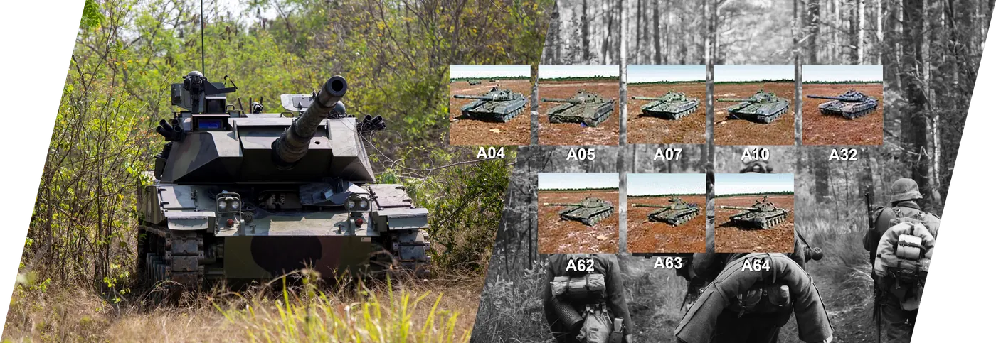
Working with data from the Sensor Data Management System (SDMS), promoted and made available by the US Air Force, is a really interesting challenge. In this case, I used the MSTAR /IU T-72 variants data.

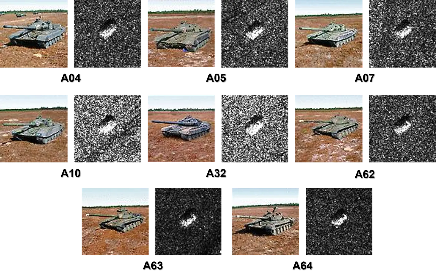
The public data in question consists of SAR (Synthetic Aperture Radar) and ISAR (Inverse Synthetic Aperture Radar) images. The sensors that produce them have an advantage when it comes to weather, since their waves pass through clouds, making it possible to obtain information without the view of the observed target being obstructed. This suits the targets provided here well: variants of the T-72 battle tank, which you can learn more about in this Wikipedia article.

There are many variants, but in this dataset there are only eight classes, as you can see below:

Setting up the environment

I needed only a few libraries for this challenge: basically Arcpy and the ArcGIS API, specifically its learn module, and finally I imported the pandas library.

from arcgis.learn import *
import arcpy
import os
import json
import pandas as pd

Preparing the data

The first step in training with ArcGIS is preparing the data. But before running the data preparation function, I had to make some adjustments to the data provided by SDMS so that it would be in the right format for the module to interpret.

So, as a first step, I had to move all the class folders for each rotation into the root image folder. After that, I just had to map the directory of each image and create the map.txt file using the function I wrote below. I also removed two images from the data folder, which I'll use to run inference with the model and test it.

dir_images= "D:\T72Variants\images"
res = os.listdir(dir_images)

lista_string = []
for sample in res:
    for path in os.scandir(dir_images + "\\"+ sample):
        if path.is_file():
            if path.name.endswith(".JPG"):
                print( "images\\"+ sample + "\\" + path.name)
                lista_string.append("images\\"+ sample + "\\" + path.name)

with open('D:\T72Variants\map.txt', 'w') as f:
    for line in lista_string:
        f.write(f"{line}\n")

After these steps, I had to change the class values and names of the images in the esri_accumulated_stats.json and esri_model_definition.emd files.

file_esri_st = open('esri_accumulated_stats.json')
file_esri_def = open('esri_model_definition.emd')
esri_st = json.load(file_esri_st)
esri_def  = json.load(file_esri_def)

new_classes = {'Classes':[{'ClassValue': 1,'ClassName': 'A04'},
                          {'ClassValue': 2, 'ClassName': 'A05'},
                          {'ClassValue': 3, 'ClassName': 'A07'},
                          {'ClassValue': 4, 'ClassName': 'A10'},
                          {'ClassValue': 5, 'ClassName': 'A32'},
                          {'ClassValue': 6, 'ClassName': 'A62'},
                          {'ClassValue': 7, 'ClassName': 'A63'},
                          {'ClassValue': 8, 'ClassName': 'A64'}]}

esri_st.update(new_classes)
esri_def.update(new_classes)

with open('esri_accumulated_stats.json', "w") as outfile:
    json.dump(esri_st, outfile)

with open('esri_model_definition.emd', "w") as outfile:
    json.dump(esri_def, outfile)

And that's it! With this, ArcGIS will be able to run the training without any problems.

For the training data preparation, I set a mini-batch size of 68 and resized the images using chip_size set to 256. For sampling, I used the stratification attribute and a random seed of 500, that is, randomly stratifying into 500 groups across the whole dataset for validation, and I set validation to 30% of the data, a percentage chosen because of the small number of samples.

data = prepare_data(out_amostras, batch_size= 68, dataset_type="ImageNet", 
                    chip_size = 256, seed = 500, val_split_pct = 0.3,
                    stratify = True)

In the end, we had 3794 images for training and 1627 images for validation.

data

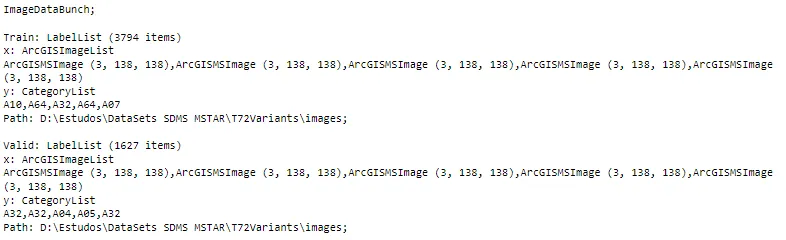
Note that even though I passed a chip_size of 256, the images have a lower resolution, 138, so the function ignored my value and used 138.

Below you can see an example of one of the batches that will be used in training.

data.show_batch()

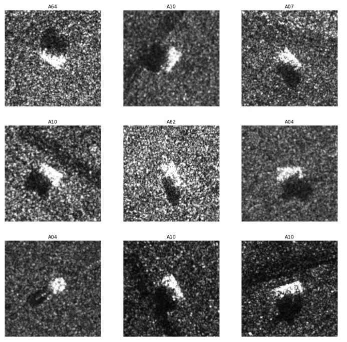
Now it was time to train the model.

Training the model

With the FeatureClassifier function, you only need to provide the dataset and the backbone architecture, in this case resnet18. I also set oversample to True since the classes and images are imbalanced, and the function will handle that problem.

model =  FeatureClassifier(data, backbone="resnet18", oversample=True)

With the model compiled, I just had to use the .lr_find (find learning rate) function, which runs iteratively and estimates the best learning rate for the deep learning model; in this case, the function found 0.0014.

lr = model.lr_find()
print("Learning Rate:",lr)

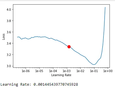
With the best Learning Rate found, I ran training for 100 epochs, but set early stopping to false, meaning the model would not stop when the gap between validation loss and train loss increased. I also enabled checkpointing, saving the best models during training.

model.fit(100, lr =lr, early_stopping=False, checkpoint=True)

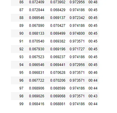
After 100 training epochs, the model reached its best accuracy of 97.48% at epoch 87, and since I had set checkpoint to True, that was the final model we used.

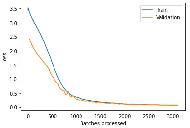
With the model finished, we can look at the loss plot, which shows that the model trained well, as both curves went down together until they reached a stable point, as expected.

model.plot_losses()

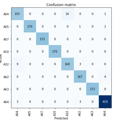
Since this is a feature classifier, it was also possible to look at the confusion matrix, which showed that most of the confusion is between classes A04 - A32, A32 - A04 and A62 - A64.

model.plot_confusion_matrix()

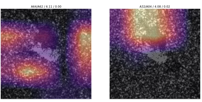
These error cases are shown when we use the .plot_hard_examples function, which displays the worst images and the Grad-CAM (Gradient-weighted Class Activation Mapping) for each of them.

model.plot_hard_examples(2)

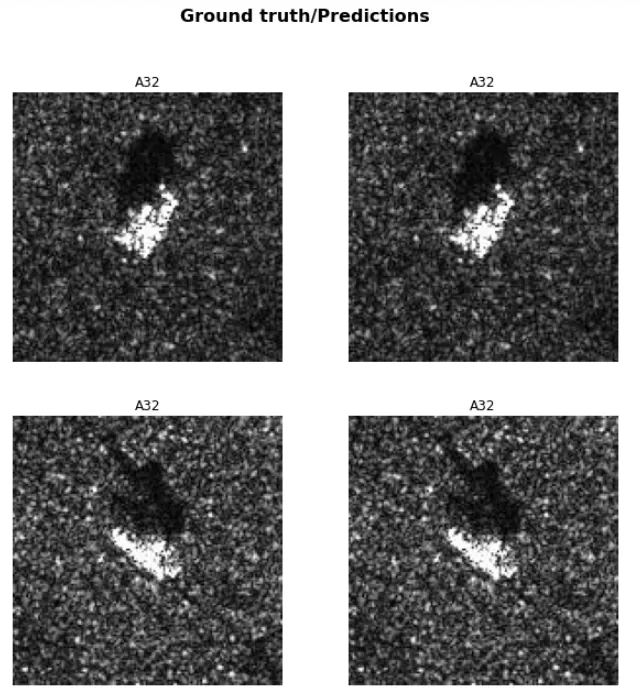
Finally, we can see the results. In this case I picked only two images, which happened to both be from class A32, and both were classified correctly.

model.show_results(2)

Predicting new images

To predict the classes of the test images, I wrote a function that searches the test images' metadata, reading the file and returning the image's class, so it can be compared with the model's prediction.

dir_teste = "D:\T72Variants\teste"

def read_metadata(diretorio):
    lista_files = []
    for path in os.scandir(dir_teste):
        if path.is_file():
            if not path.name.endswith(".JPG"):
                img_test1_char = pd.read_fwf(diretorio+path.name,
                               encoding='unicode_escape').iloc[12][0][-3:]
                lista_files.append(img_test1_char)

    return lista_files

This showed that the first and second images were A04 and A63, respectively.

read_metadata(dir_teste)

Then I ran the model's prediction using the .predict function, specifying that I wanted to visualize the output but not the gradcam.

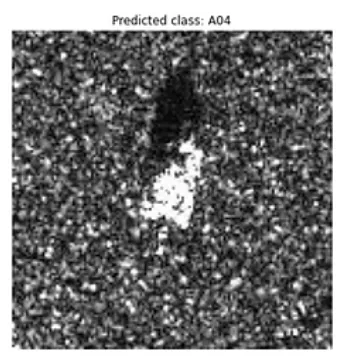
model.predict(f"{dir_teste}\\HB14937.JPG", visualize=True, gradcam=False)

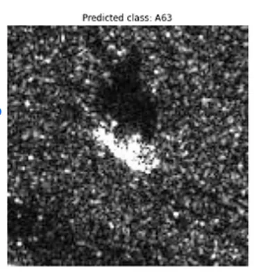
model.predict(f"{dir_teste}\\HB14961.JPG", visualize=True, gradcam=False)

This showed that the model got the class right for both test images.

Conclusion

This article once again shows the potential of ArcGIS for training deep learning models in a low-code way, which lets us focus more on tweaking parameters and experimenting than on coding the models. As shown, I trained a model with 97.48% accuracy that correctly classified both test images, with few false positives and negatives during validation.

It also demonstrates the growing potential of combining Artificial Intelligence and Remote Sensing to build effective applications and solve problems like this one in the defense sector, where information like this could guide decision-making in military tactics.

If you're interested in the Jupyter notebook where I trained the model, here is the GitHub link.